What the sampling theorem promises, where each of its assumptions fails, and what replaces it. Three articles: expert notes with error budgets and references; a general-audience summary ; and a checklist of best practices and gotchas .

Where the Sampling Theorem Stops: Failure Modes, Error Budgets, and Signal Models Beyond Band-Limiting

Chris Lomont, with Claude Fable 5.2

What this article is. The expert-level article in a pair on the sampling theorem. It goes through each hypothesis of the theorem, how it fails in practice and by how much, and the signal models that replace band-limiting, with worked numerical examples and full references. It assumes Fourier analysis and basic signal processing.

Related articles. General-audience version: What the Sampling Theorem Really Promises . Checklist: Best Practices and Gotchas . Companion topics: image resampling, dithering and quality metrics (summary ); color spaces and HDR (summary ).

Introduction

Here are notes I co-developed with Claude Fable 5.2 in October 2026 on where textbook sampling theory fails in engineering and how to address the failures. They draw on about 200 papers and books, including very recent results. Public PDFs are linked where possible; other references point to their sources.

I also wanted to show results and other directions where the usual theory is sidestepped, extended, or can be modified. Two main ideas emerge: 1) the famous rate counts degrees of freedom, not information: with noisy samples the real budget is bits, and 2) “band-limited” is one signal model among many; splines, wavelets, sparsity and parametric models each have a sampling theorem of their own.

A section of gotchas and worked examples closes the notes.

I also made a simpler summary of these notes and a short list of best practices and gotchas .

Contents

• Introduction
• 0. The short version
• 1. The theorem, its hypotheses, and its history
  • 1.1 Statement
  • 1.2 What the hypotheses actually are
  • 1.3 Priority
• 2. Failure mode I: nothing real is band-limited
  • 2.1 The obstruction
  • 2.2 Prolate spheroidal functions and the $2WT$ theorem
  • 2.3 Aliasing error bounds
  • 2.4 Aliasing in pictures
• 3. Failure mode II: the critical rate, finite records, and $\ell^\infty$ instability
  • 3.1 Exactly $2W$ is not enough for bounded signals
  • 3.2 Divergence of the Shannon series
  • 3.3 Oversampling buys a fast-decaying kernel
  • 3.4 Intersample peaks
• 4. Failure mode III: samples are not real numbers
  • 4.1 The additive-noise model and when it is exact
  • 4.2 What failure looks like
  • 4.3 Dither theory
  • 4.4 Rate against resolution
  • 4.5 Bits, not samples
• 5. Failure mode IV: time is not exact either
  • 5.1 Aperture jitter
  • 5.2 Finite aperture and the hold
  • 5.3 Ringing: the price of a sharp filter
  • 5.4 Non-linearity manufactures bandwidth
• 6. Engineering limits
  • 6.1 What bounds a converter
  • 6.2 The anti-alias filter is a system-level decision
  • 6.3 Band-pass (under)sampling
• 7. Non-uniform, multi-channel and generalized classical sampling
  • 7.1 Density is necessary: Landau
  • 7.2 Sufficient conditions and perturbations
  • 7.3 Same density, very different conditioning
  • 7.4 Irregular sampling can remove aliasing
  • 7.5 Other classical extensions, briefly
  • 7.6 Superoscillation: band-limited does not mean slowly varying
• 8. Beyond band-limiting I: other linear models
  • 8.1 Shift-invariant spaces
  • 8.2 Approximation order replaces the band edge
  • 8.3 Frames, redundancy and Balian–Low
  • 8.4 Sampling on other domains
• 9. Beyond band-limiting II: sparsity
  • 9.1 Why Fourier is the wrong language for edges
  • 9.2 Curvelets, shearlets and the geometry of edges
  • 9.3 Compressed sensing
• 10. Beyond band-limiting III: parametric signals, super-resolution, and other acquisition models
  • 10.1 Finite rate of innovation
  • 10.2 Super-resolution theory
  • 10.3 Unlimited (modulo) sampling
  • 10.4 Other acquisition models
  • 10.5 The pattern
• 11. Recent results (2020–2026)
• 12. Gotchas and teaching examples
  • 12.1 Gotchas found in the textbooks and papers
• 13. Conclusions
• References

Conventions. $\hat f(\omega)=\int f(t)e^{-i\omega t}\,dt$. $\mathrm{sinc}(t)=\sin(\pi t)/(\pi t)$. Sampling period $T$, rate $f_s=1/T$, Nyquist frequency $f_s/2$. $PW_\Omega^p$ is the Paley–Wiener space of entire functions of exponential type $\le\Omega$ whose restriction to $\mathbb R$ is in $L^p$; $PW^2_\Omega$ is the usual “finite-energy, band-limited to $|\omega|\le\Omega$”. Citations are [Author Year]; the reference list is at the end.

Status of claims. Statements are of three kinds, and the text keeps them apart:

• Cited results, with the source. Where a result could only be confirmed from memory or an abstract, the reference list flags it.
• Simulations made for this article (all figures). These are evidence about the specific examples, not proofs.
• Derivations made for this article, marked as such.

---

0. The short version

The Whittaker–Kotelnikov–Shannon (WKS) theorem is an exact statement about a model: finite-energy signals whose spectrum vanishes outside $[-\Omega,\Omega]$, infinitely many exact samples taken at exact instants, and a reconstruction filter with infinite support. Each clause fails in practice, and each failure has a quantitative theory:

Assumption	How it fails	What it costs	Section
Signal is band-limited	No time-limited signal is; real spectra decay, they do not stop	Aliasing error $\le 2\times$ out-of-band $L^1$ spectral mass; algebraic decay with rate set by smoothness	2
Infinitely many samples	Records are finite	About $2WT$ degrees of freedom, with an $O(\log WT)$ transition; truncation error $O(1/N)$ unless oversampled	2, 3
Rate exactly $2W$ is enough	True in $L^2$ only; false for bounded signals, unstable in $\ell^\infty$	Divergence in $PW^1$; unbounded intersample peaks; need a guard band	3
Samples are exact numbers	Quantized to $b$ bits, plus thermal noise	$\Delta^2/12$ only under Widrow’s conditions; otherwise distortion; information per sample is finite	4
Sampling instants are exact	Clock jitter , aperture time	SNR $\le -20\log_{10}(2\pi f\sigma_t)$, set by input frequency	5
Ideal anti-alias and reconstruction filters	Finite order, causal, or finite support	Trade among aliasing, droop, ringing, delay	5, 6
Uniform sampling	Often irregular, bunched, or missing	Landau density is necessary; conditioning can be arbitrarily bad at the same density	7
“Band-limited” is the right prior	Usually it is not: edges, transients, sparse spectra, parametric signals	A different model can need far fewer (or need different) measurements	8–10

Two themes run through everything below.

1. The $2W$ rate is a statement about degrees of freedom, not about information. With exact real-valued samples, a single sample carries infinitely many bits, and counting samples is counting dimensions. Once samples are noisy or quantized, the meaningful currency is bits (or SNR per degree of freedom), and rate can be traded against amplitude resolution in both directions: oversampled 1-bit converters reach accuracy exponential in the oversampling ratio, and at a fixed bit budget the distortion-optimal sampling rate can be below Nyquist [Kipnis 2018].

2. “Band-limited” is one subspace prior among many. WKS is the orthogonal-expansion theorem for one shift-invariant space (the one generated by sinc). Replace the generator and you get spline and wavelet sampling; replace the single subspace by a union of subspaces and you get compressed sensing , finite-rate-of-innovation sampling and super-resolution. Each alternative buys a lower measurement count and pays for it in conditioning, in model fragility, or in non-linear reconstruction. None of them repeals the degrees-of-freedom count; they change which degrees of freedom are being counted.

---

1. The theorem, its hypotheses, and its history

1.1 Statement

Theorem (WKS). If $f\in PW^2_{\pi/T}$ then

$$f(t)=\sum_{n\in\mathbb Z} f(nT)\,\mathrm{sinc}\!\left(\frac{t-nT}{T}\right),$$

with convergence in $L^2(\mathbb R)$ and uniformly on $\mathbb R$, and $\|f\|_2^2=T\sum_n|f(nT)|^2$.

Structurally: $\{\mathrm{sinc}(t/T-n)\}$ is an orthonormal basis (after scaling) of $PW^2_{\pi/T}$, and the space is a reproducing-kernel Hilbert space whose kernel is the sinc, so that point evaluation is a bounded functional and equals an inner product with a basis element: $f(nT)=\langle f,\tfrac1T\mathrm{sinc}(\cdot/T-n)\rangle$. Everything in Sections 8 –10 comes from relaxing one of the three coincidences in that sentence (orthonormal; kernel equals basis function; one linear subspace).

Shannon’s own wording [Shannon 1949, Theorem 1]: “If a function $f(t)$ contains no frequencies higher than $W$ cps, it is completely determined by giving its ordinates at a series of points spaced $1/2W$ seconds apart.” He adds that this “is a fact which is common knowledge in the communication art.”

1.2 What the hypotheses actually are

• Finite energy and a closed band. The $L^2$ theory tolerates spectral support on the closed interval because a point has measure zero. It does not cover pure sinusoids (not in $L^2$). For bounded band-limited signals (spectrum a distribution or measure supported in $[-\Omega,\Omega]$) the inequality must be strict: $\sin(\pi t/T)$ has all samples zero.
• Infinitely many samples. The sinc decays as $1/t$; every sample influences every instant.
• Exact amplitudes and exact instants. The expansion is orthonormal, so it is perfectly conditioned in $\ell^2\to L^2$. It is not bounded as a map $\ell^\infty\to L^\infty$, since $\sup_t\sum_n|\mathrm{sinc}(t-n)|=\infty$. Bounded sample errors can produce unbounded reconstruction errors (Section 3 ).
• A linear, shift-invariant model class. The set of admissible signals is a subspace, so the sum of two admissible signals is admissible. Sparse and parametric models (Sections 9 –10 ) break exactly this.

1.3 Priority

The attribution is tangled, and the surveys of Lüke and Meijering agree on the outline [Lüke 1999; Meijering 2002]:

• Borel (1897, 1899) stated the determination half and wrote down the cardinal series without the band-limited interpretation.
• E. T. Whittaker (1915) studied the cardinal function as the “simplest” interpolant through equispaced data. Lüke calls it “the first work ever to address the sampling theorem for all bandlimited functions”. Ogura (1920) gave both halves; J. M. Whittaker developed the theory in the 1920s–30s.
• Nyquist (1928) solved a different problem: the maximum rate of independent pulses through a band-limited channel, $2W$ per second. Lüke’s verdict is that Nyquist’s papers “cannot be regarded as sources for the sampling theorem”. The name “Nyquist rate ” is Shannon’s courtesy.
• Kotelnikov (1933) gave the first precise statement in a communications setting, for both low-pass and band-pass signals. Raabe (1939) treated finite-width pulses and band-pass sampling. Someya (1949) was independent of Shannon.
• Shannon (1949) used it as a lemma: $2WT$ numbers describe a signal of bandwidth $W$ and duration $T$, which turns a waveform channel into a vector channel.

For teaching: the theorem that practitioners call “Nyquist” was proved by neither Nyquist nor, first, by Shannon, and its purpose in Shannon’s paper was dimension counting.

---

2. Failure mode I: nothing real is band-limited

2.1 The obstruction

A non-zero function cannot be both time-limited and band-limited: a band-limited $f$ extends to an entire function, which cannot vanish on an interval. Every signal that starts and stops therefore has unbounded spectral support, and “band-limited” is always an approximation enforced by a filter.

Slepian’s essay On Bandwidth [Slepian 1976] makes the right move: stop asking whether a signal is band-limited and ask whether it is indistinguishable at measurement precision $\epsilon$ from one that is. Under that definition, the set of signals that are both essentially time-limited to $T$ and essentially band-limited to $W$ has approximate dimension

$$N(W,T,\epsilon)=2WT+o(WT),$$

and remarkably the leading term does not depend on $\epsilon$.

2.2 Prolate spheroidal functions and the $2WT$ theorem

The quantitative form is the Slepian–Pollak–Landau theory [Slepian 1961; Landau 1961; Landau 1962]. The operator “band-limit to $W$, then time-limit to $[-T/2,T/2]$” is compact and self-adjoint; its eigenfunctions are the prolate spheroidal wave functions and its eigenvalues $1>\lambda_0>\lambda_1>\dots>0$ are the fractions of energy that the best $k$-th function keeps inside the time window. The eigenvalues are close to 1 for $k<2WT$, close to 0 for $k>2WT$, and the transition region has width $O(\log(2WT))$:

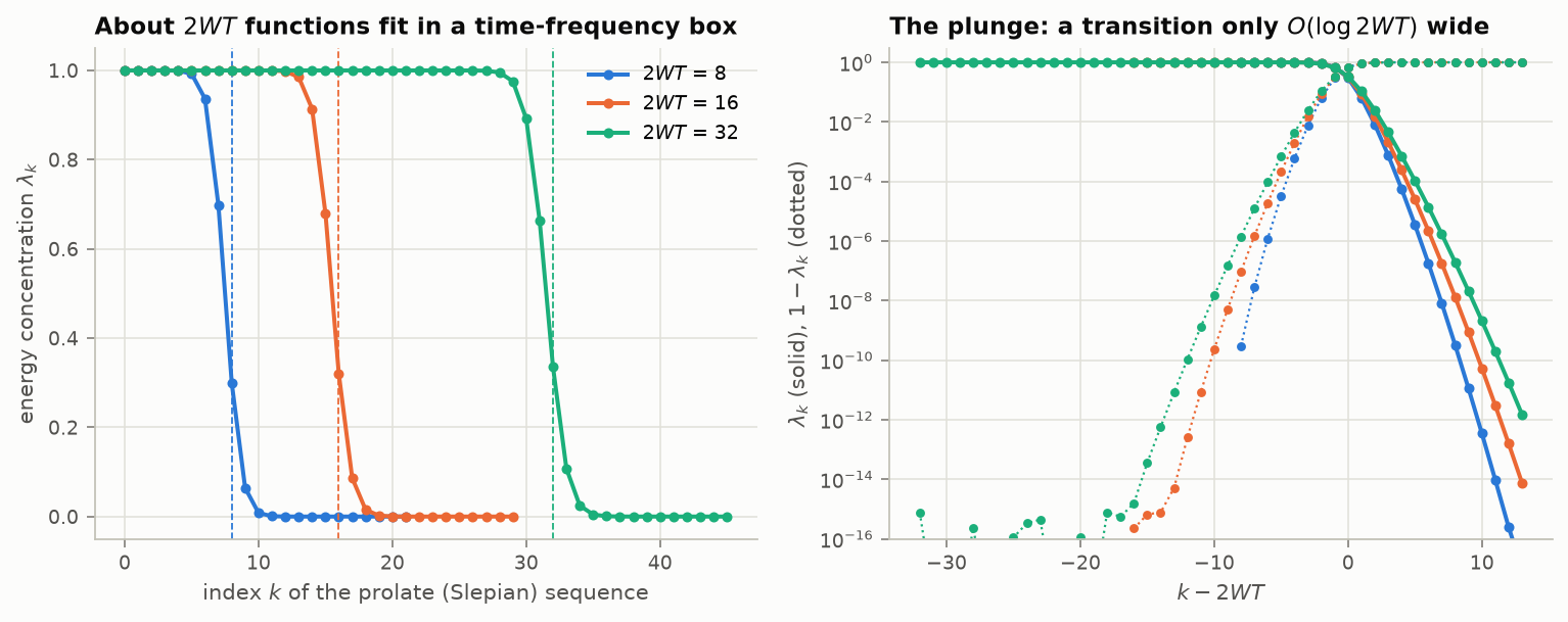
Figure 1. Discrete prolate (Slepian) sequences, record length 1024, three time–bandwidth products. Left: energy concentration $\lambda_k$ against index; the step sits at $k=2WT$ (dashed). Right: the same on a log scale, centered on $2WT$. On either side of the step the eigenvalues approach 0 or 1 exponentially, which is why “$2WT$ degrees of freedom” is a sharp statement even though no signal is exactly both limited. [Code]

Two consequences that matter later:

• The eigenvalues beyond $2WT$ are not zero, only exponentially small. Functions in that tail are band-limited, live almost entirely outside the observation window, and are nearly invisible inside it. Any attempt to recover them (extrapolation, filling long gaps, super-resolution) divides by those eigenvalues. This single fact is the source of the ill-conditioning in Sections 7.3 and 10.3 .
• The $O(\log WT)$ transition is the reason that $2WT+\text{a few}$ samples behave so much better than exactly $2WT$.

2.3 Aliasing error bounds

Sample a non-band-limited $f$ at rate $1/T$ with no prefilter and reconstruct with the sinc series. Then, with $\sigma=\pi/T$,

$$\sup_t\Big|f(t)-\sum_n f(nT)\,\mathrm{sinc}\big(\tfrac{t-nT}{T}\big)\Big|\;\le\;\frac{2}{2\pi}\int_{|\omega|>\sigma}|\hat f(\omega)|\,d\omega,$$

that is, twice the out-of-band $L^1$ spectral mass [Weiss 1963; Brown 1967; Butzer–Splettstösser 1977; statement checked against Butzer 2012]. (Butzer’s slides write it as $\sqrt{2/\pi}$ times the $L^1$ tail of the unitary-normalized transform, which is the same constant. They do not say that the constant is sharp, and neither does this article. For signals of Lipschitz order $\alpha$ in $L^2$ they give the rate $O(\sigma^{-\alpha+1/2})$, uniformly in $t$.) The factor 2 has a clean meaning: out-of-band energy does damage twice, once by being absent from where it belongs and once by reappearing, folded, where it does not belong.

In $L^2$, with an ideal prefilter the error is exactly the out-of-band energy; without one, the folded copies add. For signals whose spectrum decays like $|\omega|^{-(s+1/2)}$ (roughly, $s$ derivatives in $L^2$), both errors decay as $T^{s}$. Figure 2 shows the resulting hierarchy:

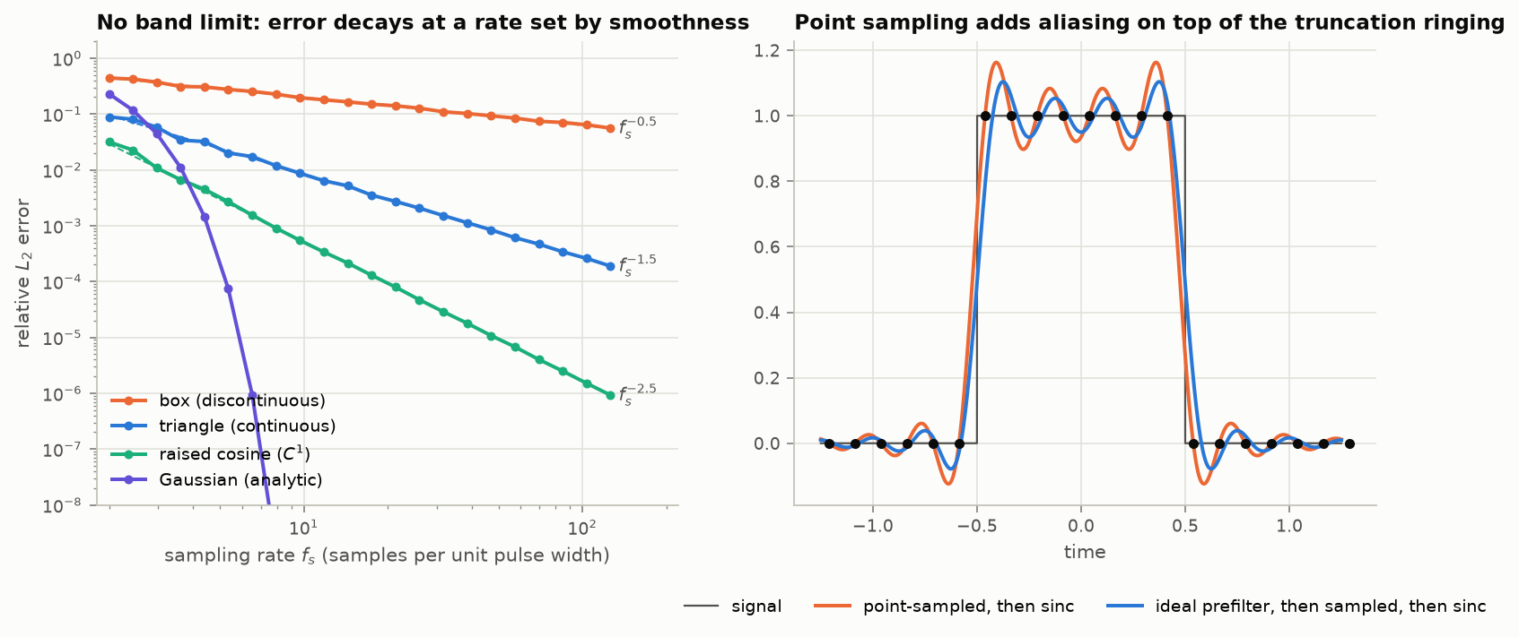
Figure 2. Left: relative $L_2$ error of “point-sample, then sinc-reconstruct” for four pulses, averaged over sampling phase. The slopes are $f_s^{-1/2}$ (box, discontinuous), $f_s^{-3/2}$ (triangle, continuous), $f_s^{-5/2}$ (raised cosine, $C^1$); a Gaussian falls faster than any power. There is no rate at which the error “switches off”. Right: the box at 8 samples per width. Even the ideal prefilter leaves Gibbs ringing (the best band-limited approximation of an edge rings); point sampling adds aliasing on top, visible as an asymmetric, phase-dependent error. [Code]

The practical reading: the sampling rate you need is set by your error tolerance and the spectral decay of the signal, not by a band edge. A discontinuous signal sampled 100× faster than its “width” is still 5% wrong in $L_2$. This is exactly the regime where other signal models win (Section 9 ).

2.4 Aliasing in pictures

Uniform sampling makes spectra periodic. Frequencies $f$ and $f\pm kf_s$ are indistinguishable from samples alone (Figure 3), and in two dimensions the aliases of a radially increasing frequency pattern appear as extra ring systems (Figure 4).

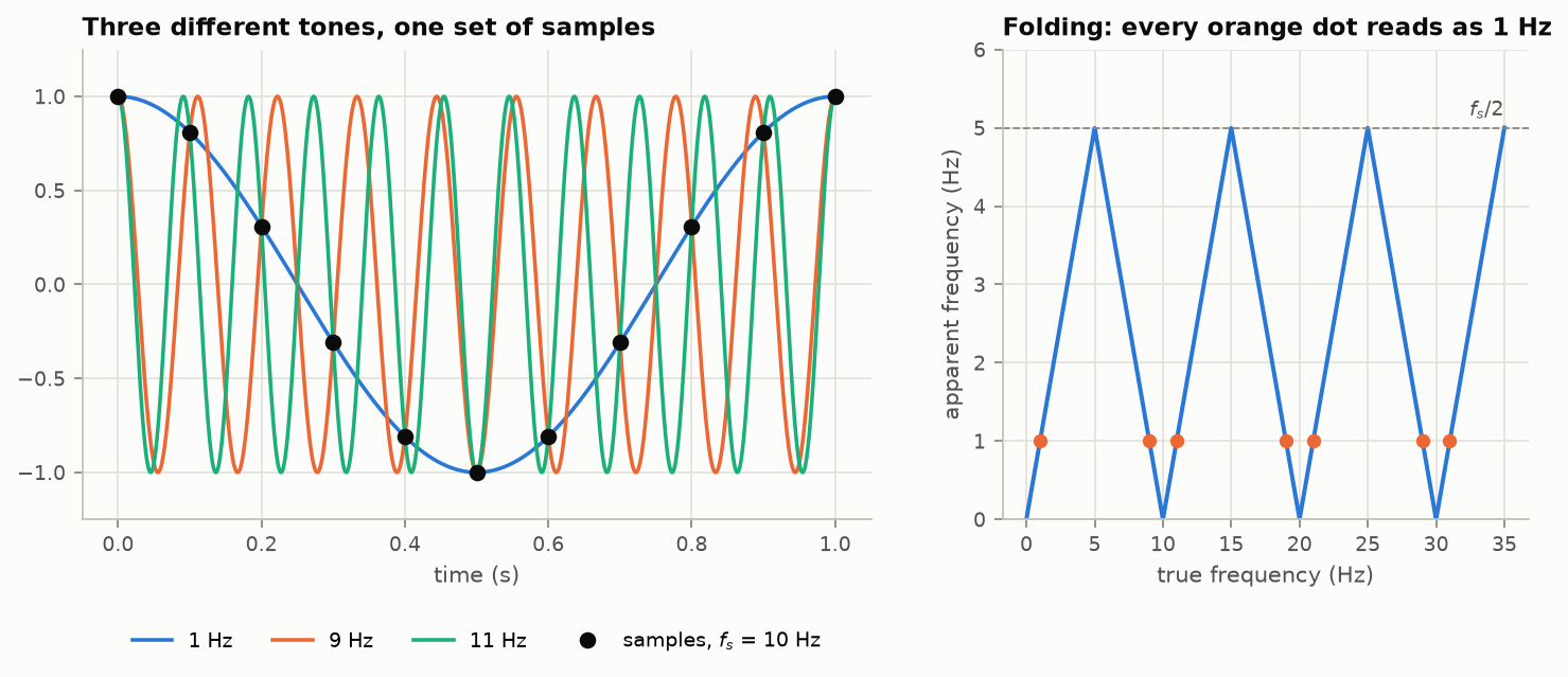
Figure 3. Left: 1 Hz, 9 Hz and 11 Hz cosines agree at every sample taken at 10 Hz. Right: apparent frequency against true frequency; every orange dot reads as 1 Hz. [Code]

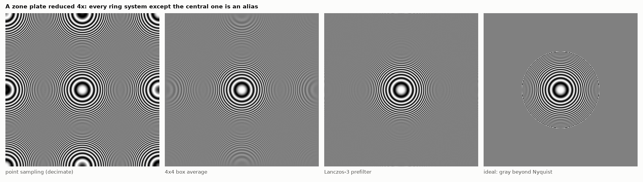
Figure 4. A zone plate (local frequency proportional to radius) reduced 4×. Point sampling reproduces the center correctly and also manufactures eight spurious ring systems, one for each neighboring spectral replica. A 4×4 box average attenuates them but its frequency response has high side lobes; Lanczos-3 does better; the ideal result is uniform gray wherever the pattern exceeds the new Nyquist frequency. View at 100%: if your viewer rescales this image it will add moiré of its own, which is the same phenomenon one level up. [Code]

---

3. Failure mode II: the critical rate, finite records, and $\ell^\infty$ instability

3.1 Exactly $2W$ is not enough for bounded signals

At $f=f_s/2$ exactly, $\sin(\pi n+\varphi)=(-1)^n\sin\varphi$: the samples carry one number, $\sin\varphi$, where two (amplitude and phase) are needed. Just below $f_s/2$ the samples are formally sufficient, but they look amplitude-modulated, and any short interpolator will reproduce that false modulation:

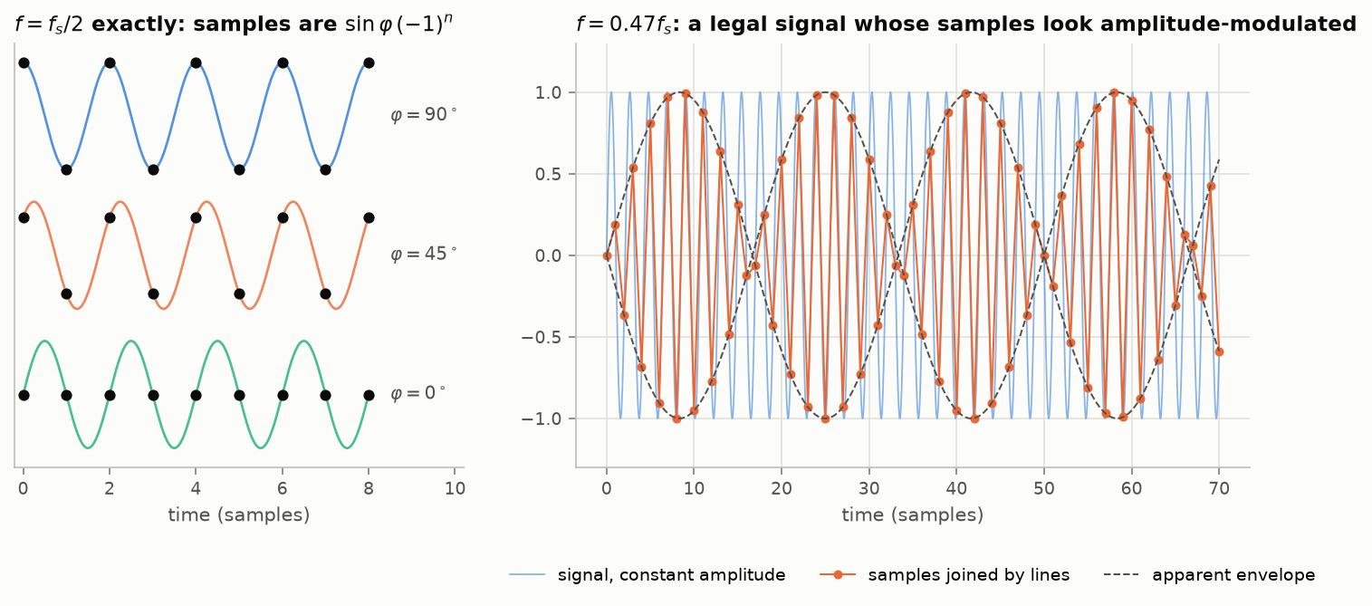
Figure 5. Left: a tone at exactly $f_s/2$; the samples see only $\sin\varphi$, and at $\varphi=0$ they are all zero. Right: a constant-amplitude tone at $0.47f_s$. The samples are sufficient in principle, but joined by straight lines they show a beat at $2(0.5-0.47)f_s$ that is not in the signal. Removing it requires an interpolator long compared with the beat period. [Code]

3.2 Divergence of the Shannon series

The $L^2$ theory hides how delicate the critical rate is. The sinc is not absolutely summable, so the sampling operator’s norm on bounded sequences is infinite. Boche and Mönich made this precise: in $PW^1_\pi$ (signals whose spectrum is merely integrable) the Shannon series converges locally uniformly, yet there exist signals for which the peak of the partial sums diverges, $\limsup_N\|S_Nf\|_\infty=\infty$ (the norms of the partial-sum operators grow at least like $C\log N$); and at the Nyquist rate no reconstruction process of the same general type is globally uniformly convergent on that space [Boche 2015; Boche–Mönich 2008, as reviewed in Boche–Pohl 2014, pp. 10–13 and 33]. Oversampling by any factor restores convergence, because then the kernel can be replaced by one that is absolutely summable.

3.3 Oversampling buys a fast-decaying kernel

If $f$ is band-limited to $Wraised cosine $t^{-3}$, a $C^\infty$ transition gives decay faster than any polynomial (never exponential, since the transform cannot be analytic and compactly supported). The classical truncation-error literature quantifies this [Helms–Thomas 1962; Jagerman 1966; Yao–Thomas 1966]: with a guard band, the truncation error of an $N$-term sum falls roughly as $1/(N\,(1-2W/f_s))$ for the plain sinc, and much faster for smooth kernels.

Figure 6 is the practical version: the error of a finite interpolation filter as a function of how close the signal comes to Nyquist.

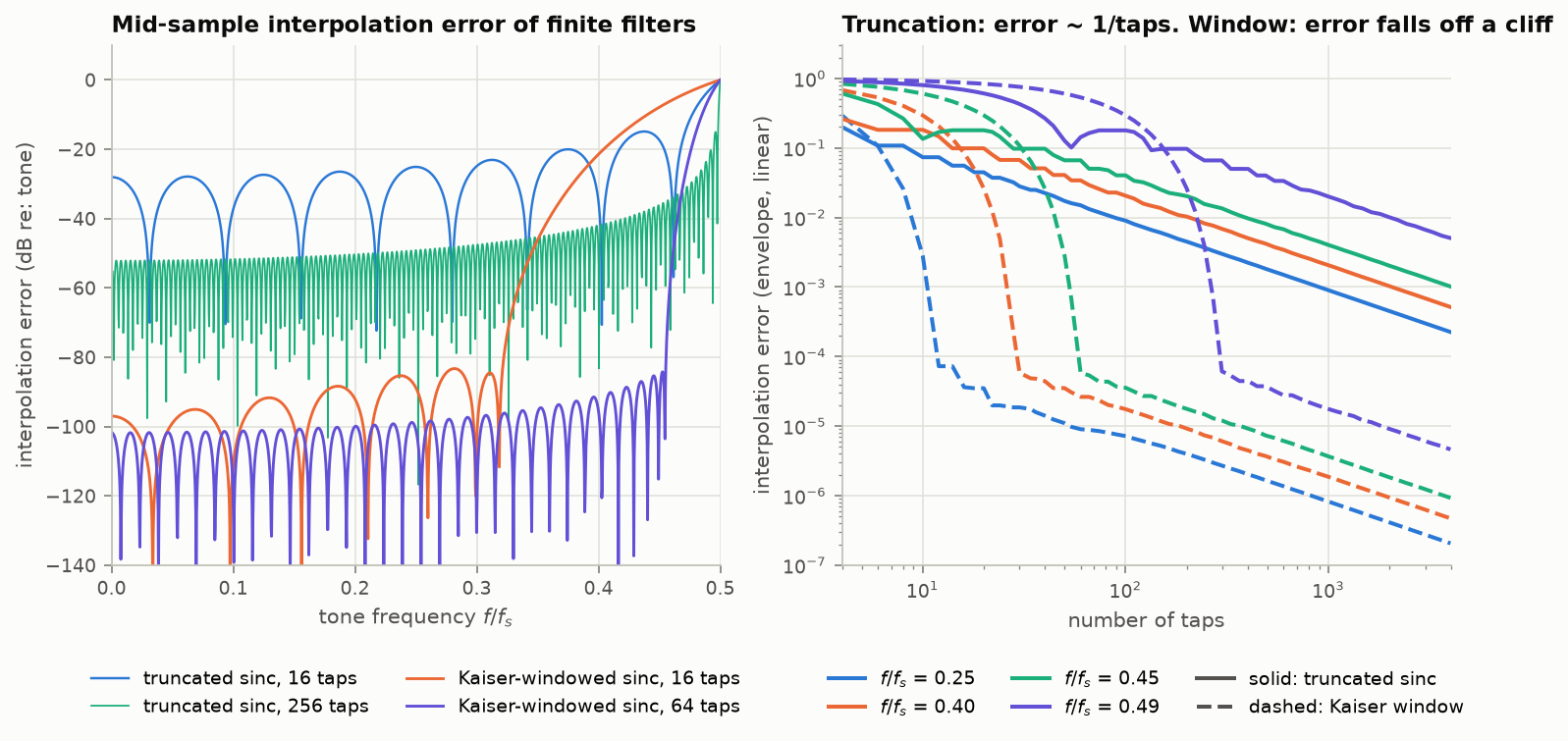
Figure 6. Error in interpolating a complex exponential at the mid-sample point. Left: against frequency. A plain truncated sinc has error that is small nowhere (about $-28$ dB with 16 taps, $-52$ dB with 256), because truncation is multiplication by a box. A Kaiser-windowed sinc of the same length is 70 dB better over most of the band, at the price of a transition band near $f_s/2$ in which it is useless. Right: against length. Truncated sinc: $O(1/\text{taps})$ at every frequency. Windowed sinc: a cliff, whose position scales as $1/(0.5-f/f_s)$; the residual floor is the window’s edge discontinuity. The engineering content of “sample faster than Nyquist” is in this panel: the guard band is what makes a short reconstruction filter possible. [Code]

3.4 Intersample peaks

The same non-summability has an audible consequence. Samples bounded by 1 do not bound the reconstructed waveform by 1. For a tone at $f_s/4$ sampled 45° off its peaks, samples of $\pm1$ correspond to a waveform peak of $\sqrt2$ (+3.01 dB). For an adversarial $\pm1$ pattern the peak is unbounded:

$$x[n]=(-1)^n\,\mathrm{sgn}\big(\tfrac12-n\big)\;\Rightarrow\; x_{\text{rec}}\big(\tfrac12\big)=\sum_{n}\frac{1}{\pi|n-\tfrac12|},$$

and truncating the pattern to $2L$ samples gives a peak of $\tfrac2\pi\sum_{k=0}^{L-1}\tfrac{1}{k+1/2}\approx\tfrac2\pi(\ln L+\gamma+2\ln2)$. This closed form was derived for this article and matches the numerics in Figure 7. It agrees with the published operator norm of the truncated Shannon series: for the partial sum $S_T$ over $|k|\le T$, $\|S_T\|=\tfrac2\pi(\ln T+2\ln2+\gamma)+O(1/T)$, with explicit two-sided bounds [Kircheis 2023, Theorem 2.2]; an earlier bound with the same leading constant is in [Trynin 2007, Theorem 1]. With oversampling the picture changes completely: for a signal of exponential type $\beta\pi$ with $\beta<1$, the peak is at most the sample peak divided by $\cos(\beta\pi/2)$ (Wunder and Boche 2003 †, as stated in [Al-Hammali 2020, Theorem 2]), a factor that grows without bound as $\beta\to1$. Daubechies and DeVore make the matching remark for sample errors: at the Nyquist rate, errors bounded by $\delta$ in a series truncated to $|n/\lambda|\le T$ cannot be held below $C\,\delta\log T$ [Daubechies 2003, p. 681].

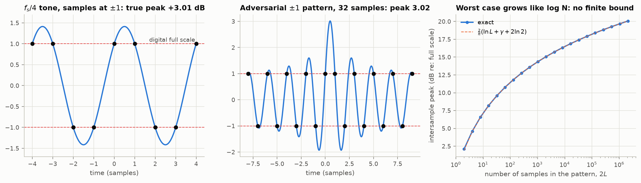
Figure 7. Left: the $f_s/4$ case, +3.01 dB. Center: the adversarial pattern with 32 samples reaches 3.02× full scale (+9.6 dB). Right: growth with pattern length, logarithmic and unbounded. This is why loudness standards specify a “true peak” measured on an oversampled signal [ITU-R 2023], and why a digital signal that never clips can clip the DAC’s reconstruction filter or a downstream sample-rate converter. [Code]

The same mechanism bounds the damage from bounded sample errors: errors of size $\varepsilon$ in $2N$ samples can produce a pointwise reconstruction error of about $\varepsilon(\tfrac2\pi\ln N+1.25)$ at the critical rate, and only $O(\varepsilon)$ with a guard band. Butzer, Splettstösser and Stens give the corresponding amplitude-error and jitter-error bounds for the cardinal series, of $\varepsilon\log(1/\varepsilon)$ type [Butzer–Splettstösser–Stens 1988].

---

4. Failure mode III: samples are not real numbers

This is the failure the theorem’s folklore handles worst. WKS says the samples determine the signal; it says nothing about what finite-precision samples determine. With exact samples, the question “how many samples per second?” has the answer $2W$. With $b$-bit samples the right question is “how many bits per second, and how should they be split between rate and resolution?”, and the answer is not $2W\times b$.

4.1 The additive-noise model and when it is exact

A uniform quantizer with step $\Delta$ has error $e=Q(x)-x\in[-\Delta/2,\Delta/2]$. The standard model treats $e$ as white, uniform, and independent of $x$, with variance

$$\sigma_e^2=\frac{\Delta^2}{12}\qquad\text{[Bennett 1948]},$$

which for a full-scale sine in a $b$-bit converter gives $\mathrm{SQNR}=6.02\,b+1.76\ \mathrm{dB}$. That formula assumes a full-scale sine, error uncorrelated with the signal, and noise integrated over the whole band to $f_s/2$.

Since $e$ is a deterministic function of $x$, independence is impossible; the model is about moments. Widrow’s observation is that quantization is sampling of the probability density: the density of $Q(x)$ is the density of $x$ convolved with a box of width $\Delta$ and then sampled on the lattice $\Delta\mathbb Z$. The characteristic function $\Phi_x(u)=E[e^{iux}]$ plays the role of the spectrum, and there is a “Nyquist condition” on it [Widrow 1996]:

• Quantizing Theorem I. If $\Phi_x(u)=0$ for $|u|>\pi/\Delta$, the density of $x$ is recoverable from the density of $Q(x)$.
• Quantizing Theorem II. If $\Phi_x(u)=0$ for $|u|>2\pi/\Delta-\epsilon$, the moments of $x$ are recoverable from those of $Q(x)$ (Sheppard’s corrections), and the error behaves as uniform noise with moments $\Delta^2/12$, $\Delta^4/80$, uncorrelated with $x$.
• Sripad–Snyder (1977). The error is exactly uniform if and only if $\Phi_x(2\pi k/\Delta)=0$ for all integers $k\ne0$, a weaker condition than QT II.

No bounded signal has a band-limited characteristic function, so these conditions never hold exactly, mirroring Section 2 . They hold approximately when the signal spans many steps with a smooth density: a Gaussian with $\sigma\ge\Delta$ has $\Phi_x(2\pi/\Delta)=e^{-2\pi^2}\approx 3\times10^{-9}$. They fail badly when the signal is small, slow, or periodic.

4.2 What failure looks like

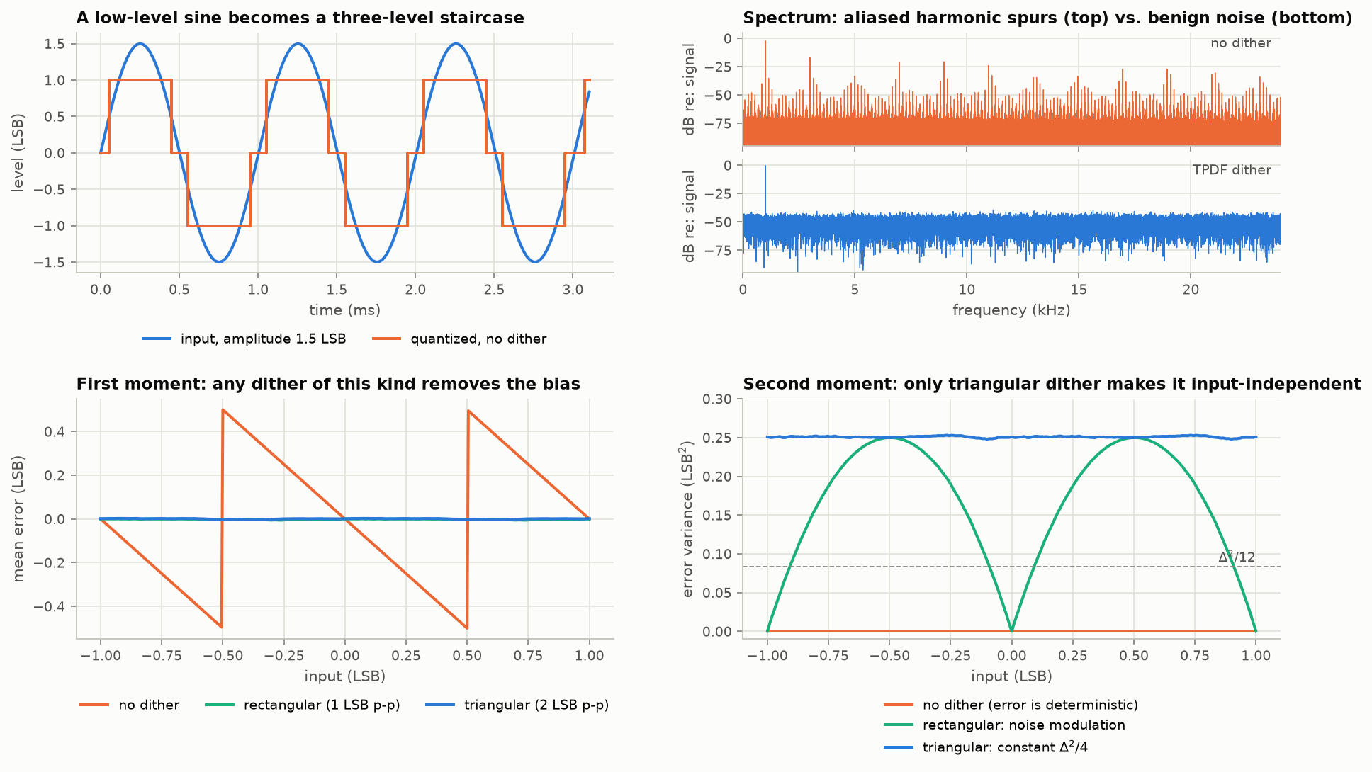
Figure 8. A 997 Hz sine of amplitude 1.5 LSB at 48 kHz. Top left: the quantizer output is a three-level staircase. Top right: its spectrum is not a noise floor but a comb of harmonics, the strongest only 17 dB below the signal, and because they extend far above $f_s/2$ they alias to frequencies with no harmonic relation to 997 Hz. Adding triangular dither replaces all of it with flat noise. Bottom: conditional moments of the total error against a static input. Any dither of at least 1 LSB peak-to-peak with the right characteristic function removes the bias. Rectangular dither leaves the error variance swinging between 0 and $\Delta^2/4$ with signal level (“noise modulation”); triangular dither makes it constant. [Code]

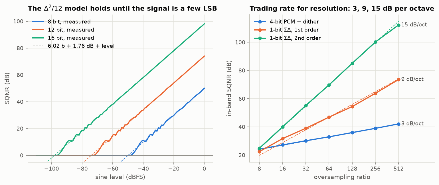
Figure 9. Left: measured SQNR of an undithered quantizer against sine level. The $6.02b+1.76$ line is followed closely until the signal is a few LSB, then departs, and below half an LSB the output is identically zero (0 dB: the error is the whole signal). Right: in-band SQNR against oversampling ratio for dithered 4-bit PCM and for 1-bit sigma-delta modulators; see 4.4. [Code]

The qualitative catalog of quantization failures:

• Harmonic and intermodulation distortion on low-level or simple periodic inputs, with the harmonics aliased.
• Vanishing signals: anything smaller than $\Delta/2$ (mid-tread) disappears.
• Noise modulation: error power that tracks the signal level.
• Limit cycles and idle tones in recursive structures (IIR filters, sigma-delta modulators with DC inputs), where the quantizer sits in a feedback loop. Figure 10’s first-order spectrum shows them.
• Granular vs. overload error: the model covers only the granular region; clipping is a separate, much worse, non-linearity.

4.3 Dither theory

Dither is the engineering use of Widrow’s condition: add an independent random signal $\nu$ before quantizing so that the total input has a characteristic function with zeros in the right places. For non-subtractive dither with total error $\varepsilon=Q(x+\nu)-x$ [Lipshitz 1992; Wannamaker 2000]:

• $E[\varepsilon^m\mid x]$ is independent of $x$ for $m=1,\dots,M$ if and only if the first $M$ derivatives of $\Phi_\nu(u)\,\mathrm{sinc}$-weighted characteristic function vanish at $u=2\pi k/\Delta$, $k\neq0$. In practice: the sum of $M$ independent rectangular variables, each 1 LSB wide, renders the first $M$ moments input-independent.
• Rectangular (RPDF, 1 LSB p-p): mean error zero for all inputs; variance still input-dependent.
• Triangular (TPDF, 2 LSB p-p): mean and variance input-independent; total error power $\Delta^2/12+\Delta^2/6=\Delta^2/4$, a 4.77 dB penalty over the undithered model figure.
• Full statistical independence of $\varepsilon$ from $x$ is unattainable with non-subtractive dither; only moments can be controlled. With subtractive dither (the receiver subtracts the same $\nu$) the error can be made genuinely independent and uniform at no noise penalty, at the cost of synchronizing the dither.

The summary engineers should carry: dither does not reduce error; it converts signal-dependent distortion into signal-independent noise, and an averaging receiver (the ear, the eye, a filter) can then recover detail below one LSB. Section 11 gives the classroom version.

4.4 Rate against resolution

Now oversample by a factor $\lambda=f_s/2W$ and ask how fast reconstruction error falls with $\lambda$ at fixed quantizer resolution.

Scheme	Reconstruction	Error decay in $\lambda$	Source
PCM (memoryless $b$-bit quantizer)	linear filtering	MSE $\Delta^2/(12\lambda)$: 3 dB per octave, half a bit per doubling	Bennett model
PCM	consistent (non-linear)	MSE $O(\lambda^{-2})$, shown by numerical tests “under certain conditions”; the proof is in the authors’ earlier work	[Thao 1994, abstract and p. 520]
Sigma-delta, order $k$, 1 bit	linear filtering	sup-norm error $O(\lambda^{-k})$ [Daubechies 2003, eq. 4 and Prop. 3.1]; MSE $O(\lambda^{-(2k+1)})$, that is $(6k+3)$ dB per octave, under the white-noise model [Thao 1994, pp. 519–520]	[Daubechies 2003; Thao 1994]
1-bit, order adapted to $\lambda$	linear filtering	$O(2^{-r\lambda})$, with $r\approx0.076$ [Güntürk 2003], then about $0.088$, now $0.102$ [Deift 2011, p. 3, checked]; any one-bit scheme has $r<1$	exponential accuracy
Any scheme using $\lambda$ bits per Nyquist interval	any	at best $O(2^{-\lambda})$, i.e. $r<1$	Kolmogorov $\varepsilon$-entropy

The first row is the precise sense in which oversampling a PCM converter is a poor trade: doubling the rate doubles the bits and buys half a bit. The third row is why delta-sigma converters dominate audio and precision measurement: a 1-bit quantizer inside a loop that shapes the error spectrum as $|1-e^{-i\omega}|^{2k}$ pushes the noise out of band, where the decimation filter removes it.

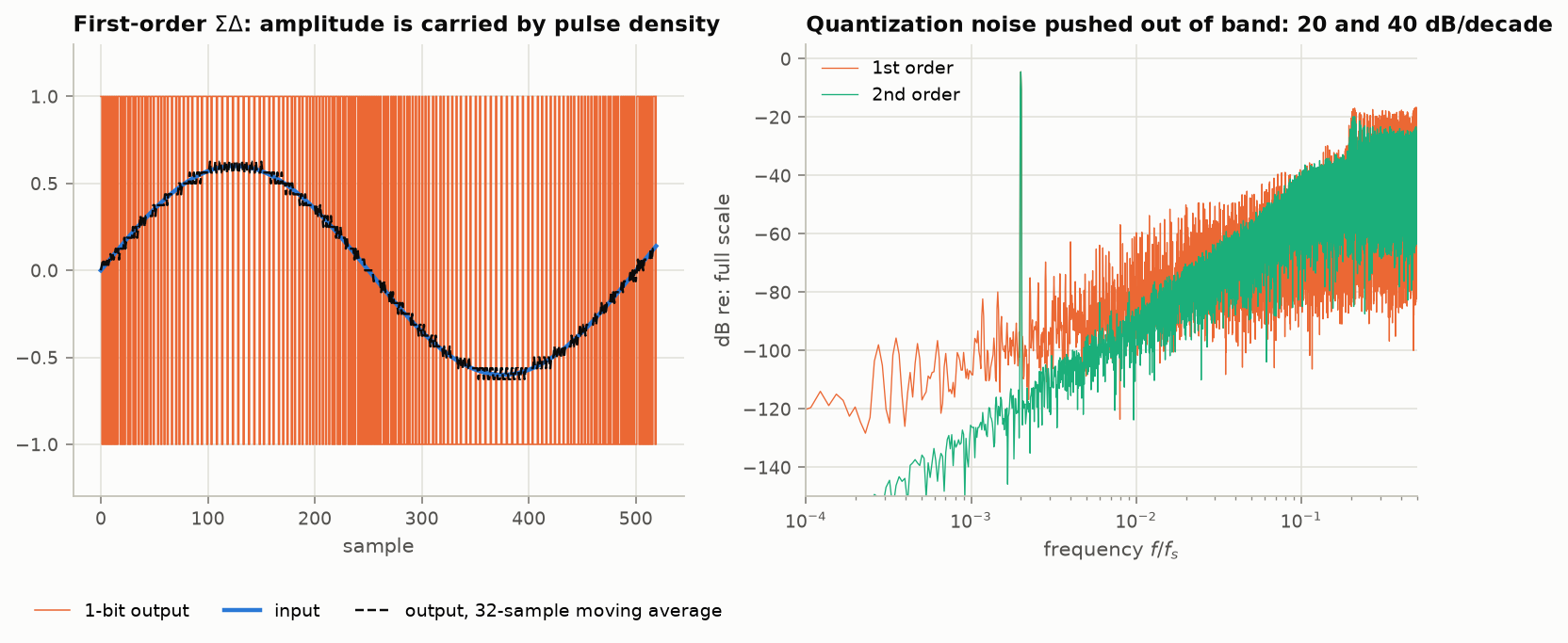
Figure 10. Left: a first-order 1-bit modulator; the sine is encoded in pulse density and a 32-sample average already tracks it. Right: output spectra. The quantization noise rises at 20 dB/decade (first order) and 40 dB/decade (second order). The first-order spectrum is visibly tonal: with a 1-bit quantizer and no dither, the “noise” is a deterministic limit-cycle structure, which is why practical converters use higher order, multi-bit quantizers, or dither. Measured slopes in Figure 9 (right): 3, 9 and 15 dB per octave, as predicted. [Code]

The last two rows of the table are the deep ones. PCM at the Nyquist rate with $b$ bits has error $2^{-b}$ and is optimal in bits, but it is not robust: its accuracy depends on comparator thresholds being exact to $2^{-b}$. Sigma-delta is robust to component error but, for a fixed order, wasteful in bits. Whether a scheme can be both exponentially accurate and robust was answered affirmatively with beta-encoders [Daubechies 2006]. This robustness-against-efficiency trade is invisible in the idealized theorem and is the real organizing principle of converter architecture.

4.5 Bits, not samples

Three results put this section in perspective.

• Capacity. A band of $W$ Hz at signal-to-noise ratio $S/N$ supports $C=W\log_2(1+S/N)$ bits per second [Shannon 1949]: $2W$ degrees of freedom per second, each worth $\tfrac12\log_2(1+S/N)$ bits. The sampling theorem supplies the first factor only. Any claim to “beat Nyquist” must be read against this: one can re-spend the $\tfrac12\log_2(1+\mathrm{SNR})$ factor, but not create capacity.
• Sub-Nyquist can be optimal under a bit budget. For a stationary Gaussian signal with a non-flat spectrum, converted at a fixed bitrate $R$, the minimum achievable distortion as a function of sampling rate is attained at a critical rate $f_R$ that is in general below the Nyquist rate; sampling faster than $f_R$ does not help [Kipnis 2018]. Intuition: reverse water-filling says the optimal code spends no bits on spectral regions whose power lies below the water level, so there is no point sampling them.
• Sampled-channel capacity. For a sub-Nyquist-sampled Gaussian channel, the optimal sampler keeps the highest-SNR frequency from each set of frequencies that alias together, and the capacity-maximizing and MSE-minimizing front ends coincide [Chen 2013].

---

5. Failure mode IV: time is not exact either

5.1 Aperture jitter

If the $n$-th sample is taken at $nT+\epsilon_n$ with $\epsilon_n$ zero-mean and rms $\sigma_t$, a sinusoid of frequency $f$ acquires an error $\approx 2\pi f A\cos(\cdot)\,\epsilon_n$, so

$$\mathrm{SNR}_{\text{jitter}}=-20\log_{10}(2\pi f\sigma_t)\qquad\text{[Neu 2010]}.$$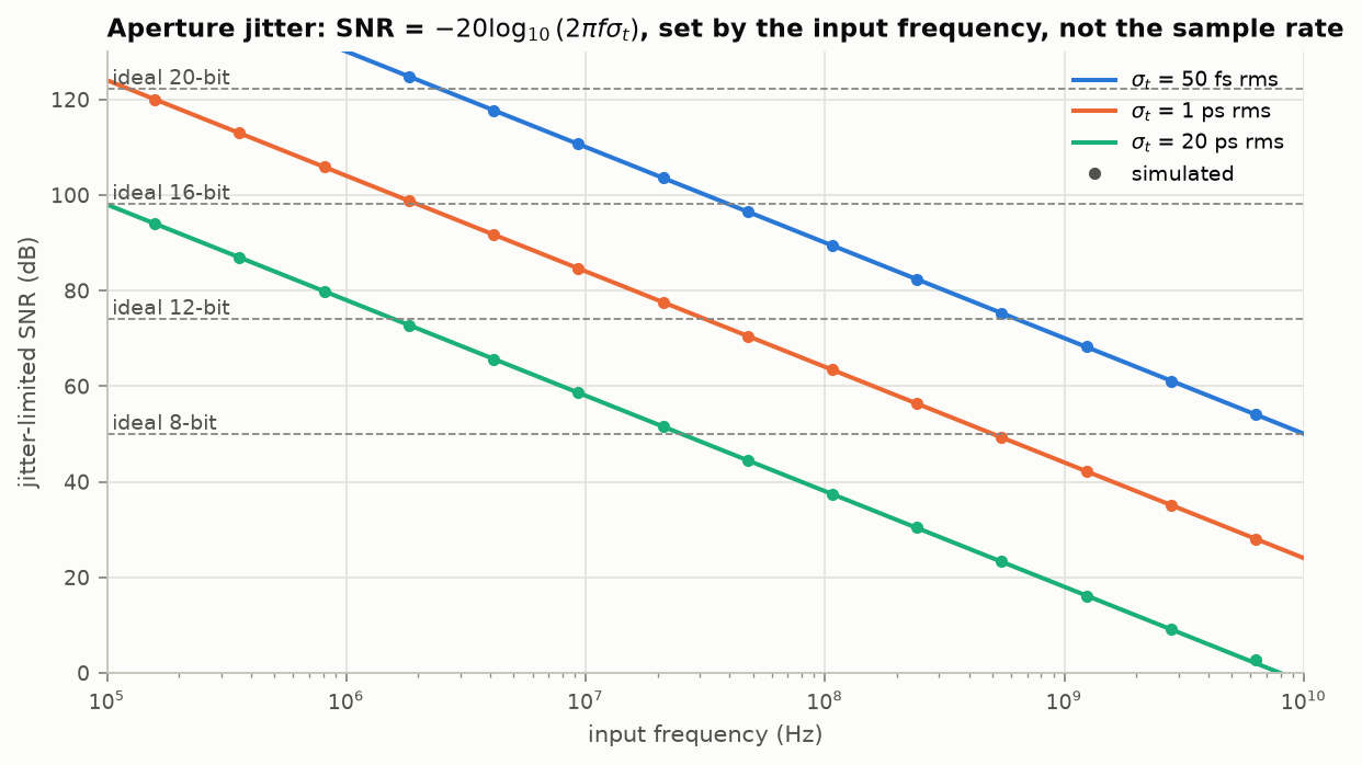

Figure 11. Jitter-limited SNR against input frequency, formula (lines) and Monte Carlo (dots), with the ideal quantization limits of 8- to 20-bit converters for reference. 1 ps rms caps a 100 MHz input at 64 dB (about 10.3 effective bits) whatever the converter’s nominal resolution. [Code]

Three points that are routinely misunderstood:

• The limit depends on the input frequency, not on the sampling rate. Undersampling a 1 GHz carrier at 100 MS/s needs a 1 GHz-quality clock.
• White jitter produces white noise, so oversampling and filtering recovers 3 dB per octave, as for PCM. Correlated jitter (close-in phase noise) instead produces skirts around each tone and is not averaged away. It can also destroy stability outright: when the timing errors follow a first-order autoregressive process, the sample set has the Landau critical density almost surely and yet almost surely is not a stable sampling set for the Paley–Wiener space; for finite records the conditioning can be bounded in terms of the record length and the jitter’s standard deviation [Gerosa 2026, abstract †].
• Jitter noise scales with signal slew, so it is signal-dependent: it vanishes for DC and is worst for the highest-frequency, highest-amplitude component.

5.2 Finite aperture and the hold

A real sampler integrates over an aperture $\tau$ (multiplying the spectrum by $\mathrm{sinc}(f\tau)$), which is a mild low-pass filter and therefore helpful as partial anti-aliasing; an image sensor’s pixel aperture is the standard example. A DAC’s zero-order hold does the same on the output side, where it is a defect:

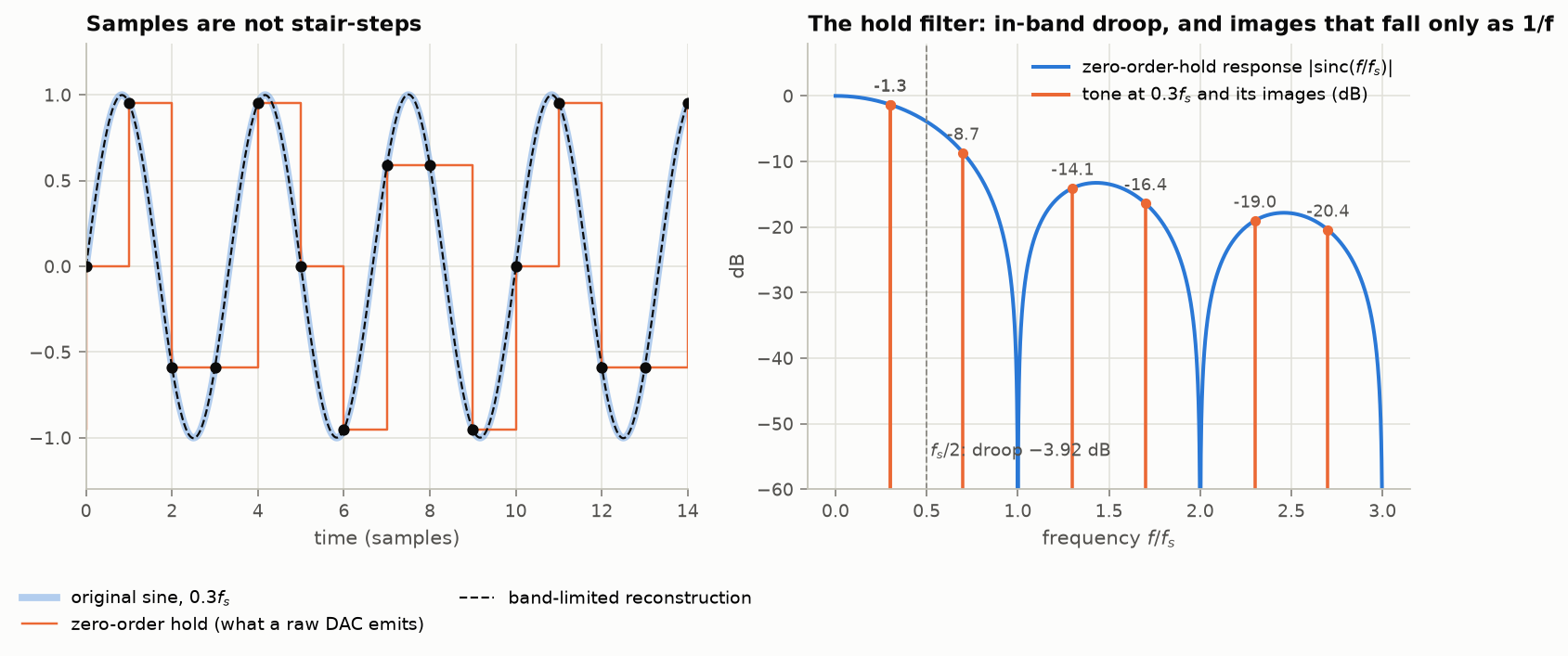
Figure 12. Left: the “stair-step” picture of digital audio conflates three things. The samples (dots) are numbers at instants; the zero-order hold (orange) is one crude reconstruction; the band-limited reconstruction (dashed) passes through the samples and coincides with the original. Right: the hold’s response, $|\mathrm{sinc}(f/f_s)|$: 3.92 dB of droop at $f_s/2$, and spectral images of every tone attenuated only by the sinc envelope ($-8.7$ dB for the first image of a tone at $0.3f_s$). The reconstruction filter’s job is to remove those images; the staircase is what the signal looks like before that filter, not after. [Code]

5.3 Ringing: the price of a sharp filter

The ideal low-pass filter’s step response overshoots by 8.949% of the step and rings at the cut-off frequency for ever, before and after the edge if the filter is linear-phase. This is not a defect of an implementation; it is what the best band-limited approximation of a step looks like.

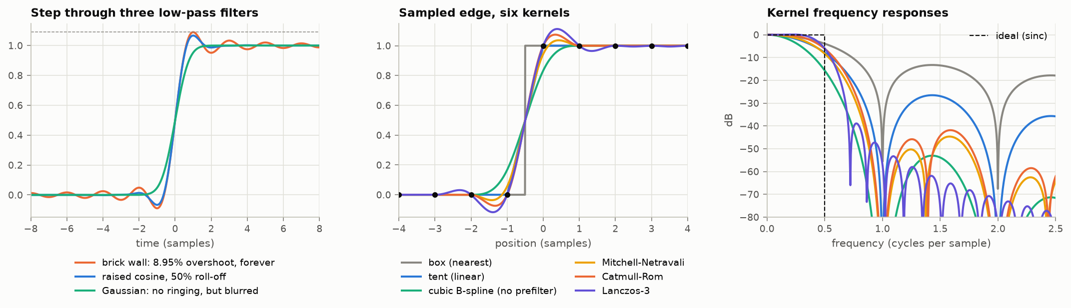
Figure 13. Left: a step through a brick-wall filter (8.95% overshoot, slowly decaying ringing), a raised-cosine roll-off (ringing dies quickly), and a Gaussian (none, but a slow edge). Center: a sampled edge reconstructed with six common kernels; negative lobes sharpen and overshoot, non-negative kernels blur. Right: their frequency responses against the ideal: pass-band droop is blur, stop-band leakage is imaging (“jaggies”). Mitchell and Netravali’s point [Mitchell 1988] is that these artifacts (blur, ringing, aliasing/imaging, anisotropy in 2-D) trade against one another and no kernel of bounded support minimizes all of them. [Code]

A filter with a transition band can ring less, which is one more reason to oversample: at 44.1 kHz the transition band from 20 kHz to 22.05 kHz forces a nearly brick-wall filter; at 96 kHz the same audio band allows a gentle one.

5.4 Non-linearity manufactures bandwidth

Sampling theory is linear; real signal chains are not. A memoryless non-linearity applied to a band-limited signal creates harmonics and intermodulation products without limit, and in a sampled system everything above $f_s/2$ folds back:

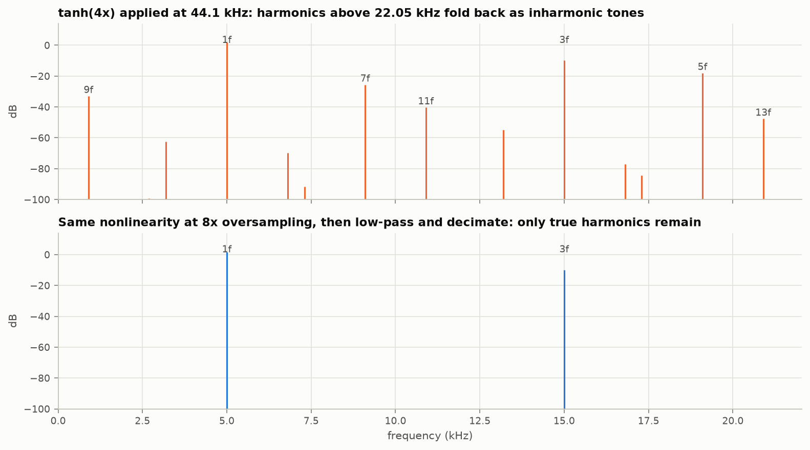
Figure 14. $\tanh(4x)$ applied to a 5 kHz sine. Top: computed at 44.1 kHz. The 5th harmonic (25 kHz) lands at 19.1 kHz, the 7th at 9.1 kHz, the 9th at 0.9 kHz, the 11th at 10.9 kHz: inharmonic tones at up to $-18$ dB. Bottom: the same operation at 8× the rate, then filtered and decimated; only the genuine harmonics below 22.05 kHz remain. The band-limited input guaranteed nothing about the output. [Code]

This is why distortion effects, compressors with fast attack, modulators, and any abs, clip or multiply in a DSP chain need internal oversampling, and why an ADC driven into clipping produces aliased products that no later filter can remove.

---

6. Engineering limits

6.1 What bounds a converter

The empirical surveys [Walden 1999; Murmann 2022] organize converter performance by which physical mechanism binds:

• Thermal noise. Sampling onto a capacitor $C$ leaves noise of variance $kT/C$, independent of the switch resistance. Requiring it not to exceed the quantization noise of a $b$-bit converter with full scale $V_{FS}$ gives $C\ge 12kT\,2^{2b}/V_{FS}^2$: each extra bit costs 4× the capacitance, and so 4× the power at a given speed. This is why high-resolution converters are slow and why the thermally limited figure of merit improves only with supply voltage and architecture.
• Wide-band noise folding. The sampler’s input bandwidth must exceed the signal bandwidth, usually by a large factor, for settling. All noise within that bandwidth folds into the first Nyquist zone. A front end with bandwidth $B$ sampled at $f_s$ raises the in-band noise density by about $2B/f_s$ relative to the unsampled circuit. An anti-alias filter is a noise filter as much as a signal filter.
• Aperture jitter, per Section 5.1 . Walden’s survey found roughly one effective bit lost per doubling of sampling rate between about 2 MS/s and 4 GS/s, which he attributed to aperture uncertainty; below about 2 MS/s converters are thermally limited. (This matches the paper’s abstract as quoted in catalogs, which adds that the figure of merit improved by about 1.5 bits over six to eight years; the full text was not obtained †.)
• Comparator ambiguity (metastability ) at multi-GS/s rates: a regenerative latch needs time proportional to $\ln(1/\text{input})$ to decide.
• Linearity (INL/DNL): static errors in the transfer curve produce harmonic spurs that, unlike noise, do not average down. Spurious-free dynamic range (SFDR) is usually the binding specification in receivers.

The summary metrics: SINAD (signal over noise plus distortion), $\mathrm{ENOB}=(\mathrm{SINAD}-1.76)/6.02$, SFDR, and figures of merit such as Walden’s $P/(2^{\mathrm{ENOB}}f_s)$ and Schreier’s $\mathrm{SNDR}+10\log_{10}\big((f_s/2)/P\big)$ [Murmann 2022, slides 8 and 62]. Two vendor notes on clock jitter, Analog Devices AN-756 and Texas Instruments SBAA653, give the jitter formula used above.

A useful sanity check for any system design: compute the three ceilings (quantization $6.02b+1.76$; jitter $-20\log_{10}2\pi f\sigma_t$; thermal) and take the lowest as a first estimate. The noise powers add, so the true figure lies somewhat below the lowest ceiling [TI SBAA653, eq. 1]. Nominal bit depth is the binding one only at low frequencies and moderate resolution.

6.2 The anti-alias filter is a system-level decision

An analog anti-alias filter must attenuate everything that would fold into the band of interest to below the noise floor. For a $b$-bit system that means roughly $6b$ dB of stop-band attenuation between the top of the pass band $W$ and $f_s-W$. The options:

• Sample barely above $2W$ and build a high-order analog filter: large group-delay variation, component sensitivity, ringing.
• Oversample heavily, use a gentle analog filter, and do the sharp filtering digitally with linear phase before decimating. This is the standard modern answer and is free in a delta-sigma converter.
• Accept some aliasing where it is benign. Image sensors do this routinely: an optical low-pass filter strong enough to suppress all aliasing would also remove wanted contrast below Nyquist.

6.3 Band-pass (under)sampling

A signal occupying $[f_L,f_H]$, bandwidth $B=f_H-f_L$, can be sampled uniformly without aliasing at any rate satisfying

$$\frac{2f_H}{n}\le f_s\le\frac{2f_L}{n-1},\qquad 1\le n\le\Big\lfloor\frac{f_H}{B}\Big\rfloor .$$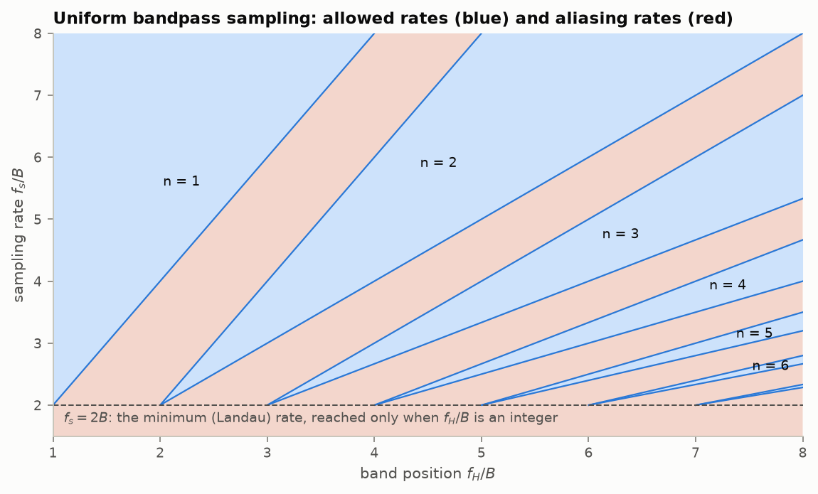

Figure 15. Allowed (blue) and forbidden (red) uniform sampling rates against band position. The minimum $f_s=2B$ is reached only at the tips of the wedges, where $f_H/B$ is an integer, and there any error in the clock or band edges causes aliasing. Vaughan, Scott and White call the minimum rate “pathological” for this reason, and note that undersampling does not preserve SNR: noise from every folded zone lands in band [Vaughan 1991]. [Code]

---

7. Non-uniform, multi-channel and generalized classical sampling

7.1 Density is necessary: Landau

For a signal whose spectrum is supported on a set $S\subset\mathbb R$ of measure $|S|$ (in Hz), any set of sampling points that permits stable reconstruction must have lower Beurling density at least $|S|$ samples per second [Landau 1967]. This Landau rate is the general form of “$2W$”: it depends on the measure of the spectral support, not on its highest frequency. Three corollaries:

• Multiband signals with known bands can be sampled at the total occupied bandwidth, though generally not with a uniform grid (periodic non-uniform patterns achieve it; Kohlenberg 1953 for a single band).
• If the band locations are unknown, the minimum rate for blind recovery of $N$ bands of width $B$ is $\min(2NB,\,f_{\text{Nyq}})$: twice the Landau rate, the factor 2 being the price of not knowing the support [Mishali 2009]. This is the same factor of 2 as “$2K$ measurements for $K$-sparse” (Section 9 ).
• No sampling scheme based on linear measurements and a subspace model can go below the Landau rate. Schemes that appear to (Section 9 –10 ) are using a non-linear model.

7.2 Sufficient conditions and perturbations

• Kadec’s $\tfrac14$ theorem. If $|\lambda_n-n|\le L<\tfrac14$ for all $n$, then $\{e^{i\lambda_nt}\}$ is a Riesz basis for $L^2[-\pi,\pi]$, so samples at the perturbed points $\lambda_n$ determine $PW_\pi^2$ stably. The constant $\tfrac14$ is sharp. Uniform sampling at exactly the critical rate therefore tolerates bounded timing perturbations below a quarter period, with a stability constant that degenerates as $L\to\tfrac14$. [Kadec 1964; stated in Bailey 2010, p. 17, and with the counterexample that shows $\tfrac14$ cannot be improved in Avantaggiati 2016, Theorem 7].
• Papoulis’ generalized sampling expansion. A band-limited signal is determined by the outputs of $M$ independent linear filters each sampled at $1/M$ of the Nyquist rate: the signal and its derivative at half rate, interleaved offset combs, and so on [Papoulis 1977]. Total rate is unchanged; what changes is conditioning, which can be very poor [Cheung–Marks 1985; Unser 1997].
• Frames. A sampling set is stable exactly when the corresponding exponentials (or kernel translates) form a frame; oversampling makes the frame redundant, and reconstruction with the canonical dual averages white noise down by the redundancy factor.

7.3 Same density, very different conditioning

The Landau rate is necessary and, with exact data, often sufficient. It says nothing about noise amplification. Two computed examples:

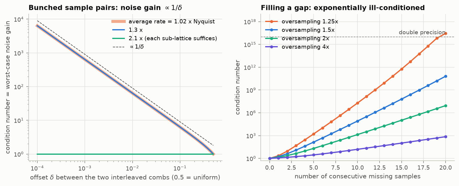
Figure 16. Left: a trigonometric polynomial sampled on two interleaved uniform combs offset by $\delta$ (recurrent non-uniform sampling). The average rate never changes. Near the minimum rate the condition number of the reconstruction grows as $1/\delta$: as the two combs approach, each pair of samples measures the signal and (nearly) its derivative, and the derivative is obtained by dividing a small difference by a small $\delta$. At 2.1× the minimum rate each comb suffices alone and bunching is harmless. Right: a uniform, oversampled record with a run of consecutive samples missing. The missing samples are determined in principle, but the condition number grows exponentially with the length of the gap, at a rate that falls with the oversampling ratio; at 1.25× oversampling, 20 missing samples exhaust double precision. This is Figure 1’s exponentially small eigenvalues, met from the other side. [Code]

The engineering translation: time-interleaved ADCs with timing skew, sensor arrays with clustered elements, and “we will just interpolate the dropouts” all live on these curves.

7.4 Irregular sampling can remove aliasing

Uniform sampling aliases coherently: an out-of-band tone becomes a clean in-band tone. Irregular sampling has no single Nyquist frequency. For sample times on a lattice of pitch $p$ (the largest $p$ such that all time differences are multiples of $p$) the true folding frequency is $1/(2p)$, which for timestamps of finite precision is far above the mean-rate figure [Eyer 1999]; and the commonly quoted “pseudo-Nyquist” limits based on mean or minimum spacing are simply wrong [VanderPlas 2018].

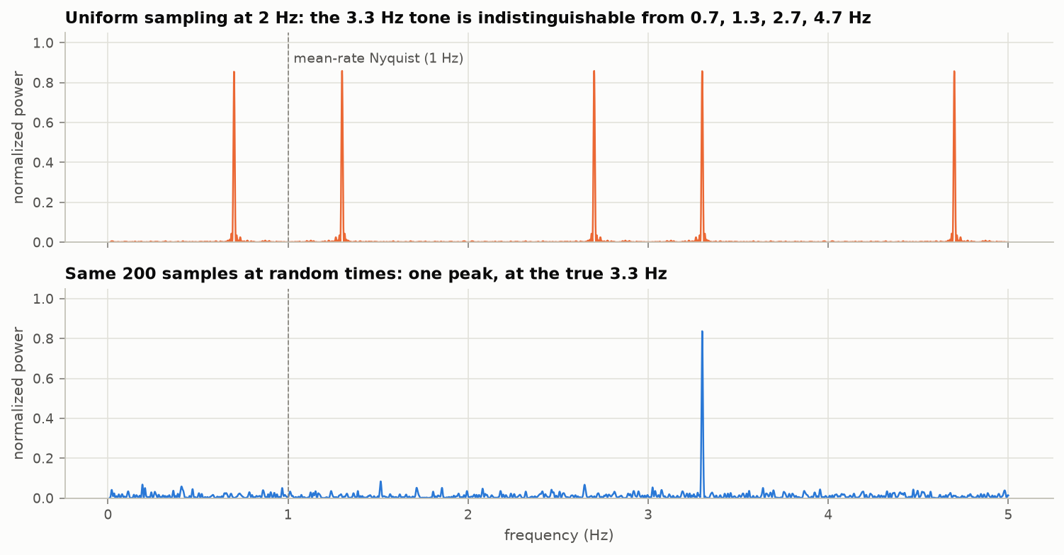
Figure 17. A 3.3 Hz tone in noise, 200 samples over 100 s. Sampled uniformly at 2 Hz, its periodogram has identical peaks at 0.7, 1.3, 2.7, 3.3 and 4.7 Hz. Sampled at 200 random times with the same mean rate, there is one peak, at the true frequency; the alias energy has been spread into a noise-like floor. [Code]

The same idea is the basis of stochastic sampling in rendering (Figure 18) and of the random sampling patterns in compressed sensing (Section 9.3 ). It is not free: the alias energy is still there, as broadband noise, and reconstruction of the waveform (as opposed to detection of a few tones) still needs the Landau density.

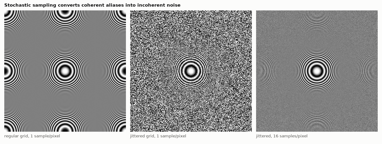
Figure 18. A zone plate point-sampled on a regular grid (structured moiré), on a jittered grid (the same error energy as unstructured noise), and with 16 jittered samples per pixel. The eye tolerates the noise far better than the false structure. Residual rings in the right panel are aliases that the 1-pixel box filter does not remove. [Code]

7.5 Other classical extensions, briefly

• Derivative sampling, Hermite-type expansions: special cases of Papoulis.
• Zero-crossings. A band-pass signal of less than one octave bandwidth, having no zeros in common with its Hilbert transform other than real simple ones, is determined up to scale by its real zero crossings [Logan 1977]. A striking uniqueness theorem and a practical dead end: Logan’s own abstract says that recovery “appears to be very difficult and impractical”.
• Kramer’s theorem and other kernels: sampling expansions for transforms other than Fourier (Hankel, Legendre, fractional Fourier, linear canonical), each with its own notion of “band-limited”.
• Lattices in several dimensions: for isotropically band-limited 2-D signals the hexagonal lattice needs 13.4% fewer samples than the square one (Petersen and Middleton 1962); on the sphere, exact quadrature for band-limit $L$ needs about $2L^2$ samples on an equiangular grid although the space has dimension $L^2$ [McEwen 2011].

7.6 Superoscillation: band-limited does not mean slowly varying

A band-limited function can oscillate arbitrarily fast on an arbitrarily long interval. A standard example with all frequencies in $[-1,1]$:

$$f(x)=\Big(\cos\tfrac{x}{N}+i\,a\sin\tfrac{x}{N}\Big)^{N},\qquad a>1,$$

which near $x=0$ behaves like $e^{iax}$.

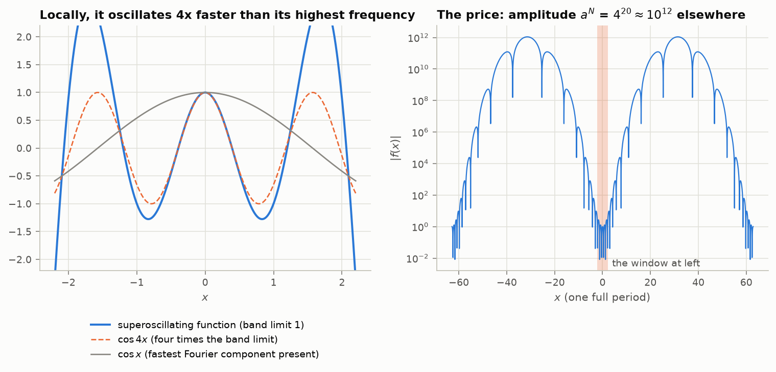
Figure 19. $N=20$, $a=4$. Left: near the origin the function follows $\cos4x$, four times faster than its highest Fourier component. Right: the cost. Outside the superoscillating window the amplitude reaches $a^N\approx10^{12}$. The energy cost grows exponentially with the number of superoscillations [Ferreira–Kempf 2006; Kempf 2018]. [Code]

Superoscillations are the synthesis-side face of the tail eigenvalues in Figure 1 and the analysis-side ill-conditioning of super-resolution in Section 10.3 . They also dispose of a common intuition: local sample spacing cannot be chosen from “local bandwidth” in any naive sense, because a band-limited signal’s local behavior is unconstrained if one is willing to pay in dynamic range .

---

8. Beyond band-limiting I: other linear models

8.1 Shift-invariant spaces

Unser’s fifty-year retrospective [Unser 2000] reframes sampling as approximation in a shift-invariant space

$$V_T(\varphi)=\Big\{\sum_k c_k\,\varphi\big(\tfrac{t}{T}-k\big):c\in\ell^2\Big\},$$

where the generator $\varphi$ need only satisfy a Riesz condition $0B-spline of degree $n$) gives splines; a scaling function gives a multiresolution space. Three things change relative to WKS and all three are improvements for real systems:

1. The measurement need not be a point sample. An acquisition device computes $c_1[k]=\langle f,\varphi_1(\cdot/T-k)\rangle$ for some analysis function $\varphi_1$ (the impulse response of the sensor: a pixel aperture, a sample-and-hold, an optical point-spread function). The ideal prefilter in WKS is the special case $\varphi_1=\mathrm{sinc}$.
2. Reconstruction is in a space you choose, $V(\varphi_2)$, typically with a compactly supported generator.
3. A digital correction filter joins them. Demanding consistency (re-measuring the reconstruction returns the same samples) gives $\tilde f=\sum_k (c_1{\ast}q)[k]\,\varphi_2(t-k)$ with $$Q(e^{i\omega})=\Big[\sum_k\overline{\hat\varphi_1(\omega+2\pi k)}\,\hat\varphi_2(\omega+2\pi k)\Big]^{-1},$$ and $\tilde f$ is the oblique projection of $f$ onto $V(\varphi_2)$ along $V(\varphi_1)^\perp$ [Unser 1994]. Its error is within a factor $1/\cos\theta_{12}$ of the best possible (the orthogonal projection), where $\theta_{12}$ is the angle between the two spaces. For box-shaped analysis and spline synthesis this factor is about 1.15–1.3, i.e. almost nothing is lost by using the sensor you have rather than the ideal prefilter.

The message for practice: the anti-alias filter, the sampler and the reconstruction filter are one design problem, and the classical “ideal low-pass, then point-sample, then ideal low-pass” is merely the solution for one choice of spaces. Nehab and Hoppe’s monograph develops this for graphics and makes the digital filter $q$ a first-class pipeline stage [Nehab 2014]; Eldar and Michaeli extend it to smoothness priors, minimax criteria and non-linear distortions [Eldar 2009].

8.2 Approximation order replaces the band edge

A non-band-limited signal has no Nyquist rate. What it has, in a given space, is a rate of convergence as $T\to0$:

$$\|f-P_Tf\|_{L^2}\le C_\varphi\,T^{L}\,\|f^{(L)}\|_{L^2},$$

where $L$ is the approximation order of $\varphi$. By the Strang–Fix conditions, $L$ is the number of polynomial degrees that integer shifts of $\varphi$ reproduce, equivalently the order of the zeros of $\hat\varphi$ at $2\pi k$, $k\ne0$. A B-spline of degree $n$ has $L=n+1$; Keys’ cubic has $L=3$; the sinc has $L=\infty$, which is the precise sense in which it is “ideal” and also the reason it is not a sensible target for signals that are not smooth.

Blu and Unser’s error kernel gives the whole picture rather than the asymptote [Blu 1999]:

$$\|f-Q_Tf\|^2\approx\frac1{2\pi}\int|\hat f(\omega)|^2\,E(T\omega)\,d\omega,\qquad E_{\min}(\omega)=1-\frac{|\hat\varphi(\omega)|^2}{\sum_k|\hat\varphi(\omega+2\pi k)|^2},$$

exact when averaged over all shifts of the input. Sampling quality becomes a single integral of the signal’s power spectrum against a kernel fixed by the method, and methods can be compared (and optimized) on that basis. This is how O-MOMS (maximal order, minimal support, optimized constant) and the optimized quasi-interpolators were designed.

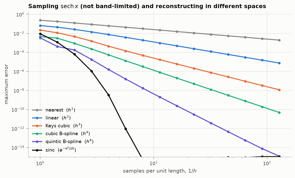
Figure 20. Maximum error in reconstructing $\mathrm{sech}\,x$ (analytic, not band-limited) from samples at spacing $h$. Each method follows its order: $h$, $h^2$, $h^3$, $h^4$, $h^6$. The sinc series converges exponentially here because the spectrum decays exponentially; for a signal with a kink it would be no better than the others and would ring. A cubic B-spline reaches $10^{-6}$ with about 10 samples per unit length using a 4-tap kernel plus a one-pole recursive prefilter. [Code]

8.3 Frames, redundancy and Balian–Low

A stable sampling set corresponds to a frame, $A\|f\|^2\le\sum_k|\langle f,f_k\rangle|^2\le B\|f\|^2$ (Duffin and Schaeffer, 1952, introduced frames for exactly this purpose: non-harmonic Fourier series, i.e. non-uniform sampling). Redundancy $r$ averages white coefficient noise down by $1/r$, gives robustness to erasures, and (Section 4.4 ) converts into amplitude resolution.

For time–frequency (Gabor) systems $\{e^{2\pi ibmt}g(t-an)\}$ there is a sharp density theorem: a frame requires $ab\le1$, completeness fails for $ab>1$, and at the critical density $ab=1$ the Balian–Low theorem forbids a window that is well localized in both time and frequency. This is the time–frequency analog of Section 3 : critical sampling is possible only with a badly behaved kernel, and a modest redundancy removes the obstruction.

8.4 Sampling on other domains

The same template (a “band-limited” subspace defined by an operator’s low eigenspace, plus a stable sampling set) has been carried to graphs (Laplacian eigenvectors [Chen 2015; Anis 2016; Tanaka 2020]), simplicial complexes [Barbarossa 2020], the sphere [McEwen 2011] and manifolds. The new difficulty there is choosing the sampling set, since there is no lattice.

---

9. Beyond band-limiting II: sparsity

9.1 Why Fourier is the wrong language for edges

Band-limiting is a linear model: keep the first $N$ Fourier coefficients. Its error for a signal with $s$ derivatives decays like $N^{-s}$. A single jump destroys this: Fourier coefficients of a discontinuous function decay as $1/k$, so the squared error of the best $N$-term approximation, linear or not, is stuck at $N^{-1}$.

Wavelets with enough vanishing moments have coefficients that are small wherever the signal is locally smooth, so a jump costs only $O(1)$ large coefficients per scale. Keeping the $N$ largest coefficients (a non-linear, signal-adapted choice) restores the smooth rate:

Signal class	Fourier	Wavelets, best $N$ terms	Optimal
1-D, piecewise $C^s$ (squared $L^2$ error)	$N^{-1}$	$N^{-2s}$	$N^{-2s}$
2-D “cartoon”: $C^2$ regions, $C^2$ edges	$N^{-1/2}$	$N^{-1}$	$N^{-2}$
same, curvelets / shearlets		$N^{-2}(\log N)^3$

[DeVore 1998; Candès 2004; Kutyniok 2011; Mallat, Wavelet Tour, ch. 9.]

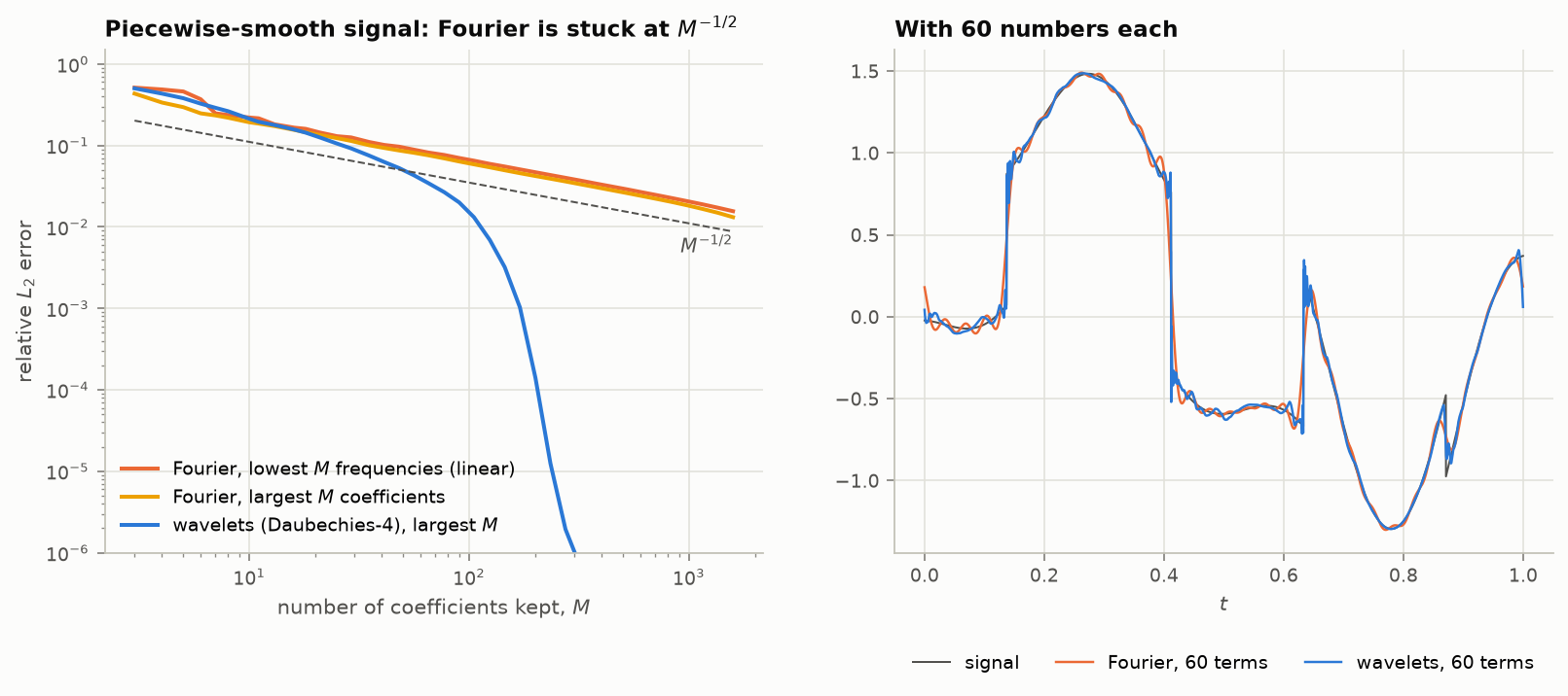
Figure 21. A piecewise-smooth signal with four jumps. Left: relative $L_2$ error against the number of coefficients kept. Fourier follows $M^{-1/2}$ whether one keeps the lowest frequencies or the largest coefficients. Wavelets start no better and then fall away steeply once $M$ exceeds roughly (jumps) × (scales) × (filter length), the number of coefficients the edges actually occupy. Right: 60 terms each; the Fourier approximation rings along its whole length, the wavelet one errs only at the jumps. [Code]

The right smoothness scale is correspondingly different. Linear approximation at rate $N^{-s}$ characterizes Sobolev spaces; non-linear $N$-term wavelet approximation at the same rate characterizes the much larger Besov spaces $B^s_\tau(L_\tau)$, $1/\tau=s/d+1/2$, which contain functions with jumps [DeVore 1998]. Donoho’s formulation: an unconditional basis for a function class is the optimal basis for compressing it and for estimating it in noise, and thresholding in that basis is near-minimax [Donoho 1998].

9.2 Curvelets, shearlets and the geometry of edges

In two dimensions wavelets are themselves sub-optimal, because an edge is a curve: an isotropic wavelet of scale $2^{-j}$ meets it in $\sim2^{j}$ places, so the number of significant coefficients grows geometrically with scale and the squared error decays only as $N^{-1}$. Curvelets [Candès 2004] are a tight frame of anisotropic, oriented elements obeying parabolic scaling (width ≈ length²), so that one element can lie along a $C^2$ edge. They achieve $N^{-2}(\log N)^3$, the optimal rate up to the logarithm, without adapting to the image. Shearlets reach the same rate with compact support and a cleaner discretization [Kutyniok 2011]; contourlets are a filter-bank construction with the same aim [Do 2005]; bandlets and wedgelets get there by explicit adaptation to edge geometry; wave atoms are tuned to oscillatory textures.

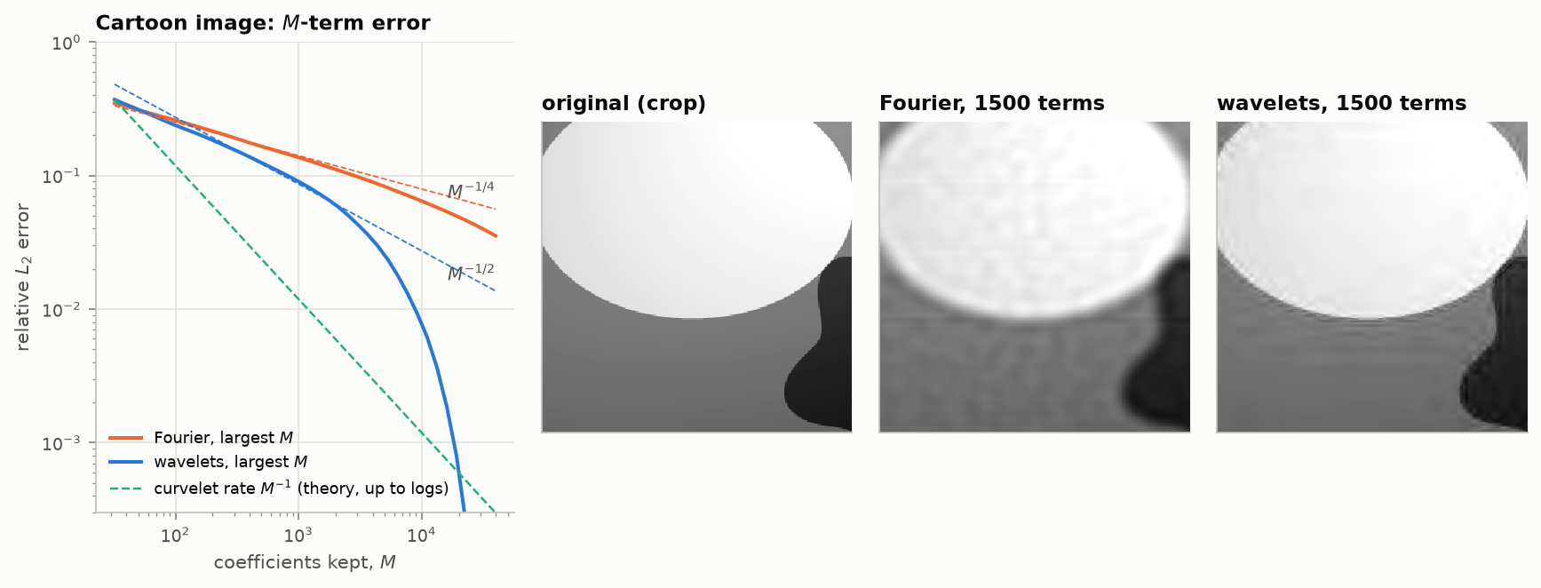
Figure 22. A cartoon image (smooth regions, smooth edges). Left: $M$-term error. Fourier follows $M^{-1/4}$ and wavelets $M^{-1/2}$ in $L_2$ norm (the square roots of the rates in the table), until the discrete image’s finite resolution takes over; the dashed green line is the curvelet rate, shown for reference and not computed. Right: 1500 coefficients each. Fourier spends them on global ringing; wavelets keep edges sharp. [Code]

Where these fit in a discussion of sampling: they are statements about how many numbers describe a signal to a given accuracy, which is the question the sampling theorem answers for the band-limited class. They do not by themselves tell you how to acquire those numbers without first acquiring everything. That is the contribution of the next section.

9.3 Compressed sensing

If a length-$n$ signal is $k$-sparse in a known basis, $k$ numbers describe it, but which $k$ is unknown. The set of $k$-sparse signals is a union of $\binom nk$ subspaces, not a subspace. Lu and Do’s framework [Lu 2008] gives the linear-algebra core: a linear measurement map is injective on the union if and only if it is injective on every sum of two member subspaces, so at least $2k$ measurements are needed; the factor 2 is the price of not knowing the support, and is the same factor as “twice the Landau rate” for blind multiband sampling.

The compressed-sensing theorems say that about $k\log(n/k)$ non-adaptive, random linear measurements suffice, with recovery by convex optimization:

• Exact recovery from random frequency samples [Candès 2006a]: $|T|\le C\,|\Omega|/\log n$ suffices with high probability for $\ell_1$ minimization to recover a signal supported on $T$ from its Fourier coefficients on a random set $\Omega$.
• Stability via the restricted isometry property [Candès 2008]: if $\delta_{2s}<\sqrt2-1$, the $\ell_1$ solution satisfies $\|x^\star-x\|_2\le C_0s^{-1/2}\|x-x_s\|_1+C_1\varepsilon$: graceful degradation with both compressibility and noise.
• Sharp phase transition [Donoho 2009]: for Gaussian matrices, success and failure are separated by a curve in the $(m/n,\,k/m)$ plane, now understood exactly through the statistical dimension of the $\ell_1$ descent cone.
• Lower bound: stable recovery of all $k$-sparse vectors needs $m\gtrsim k\log(n/k)$ (Gelfand widths), so the logarithm is not an artifact.

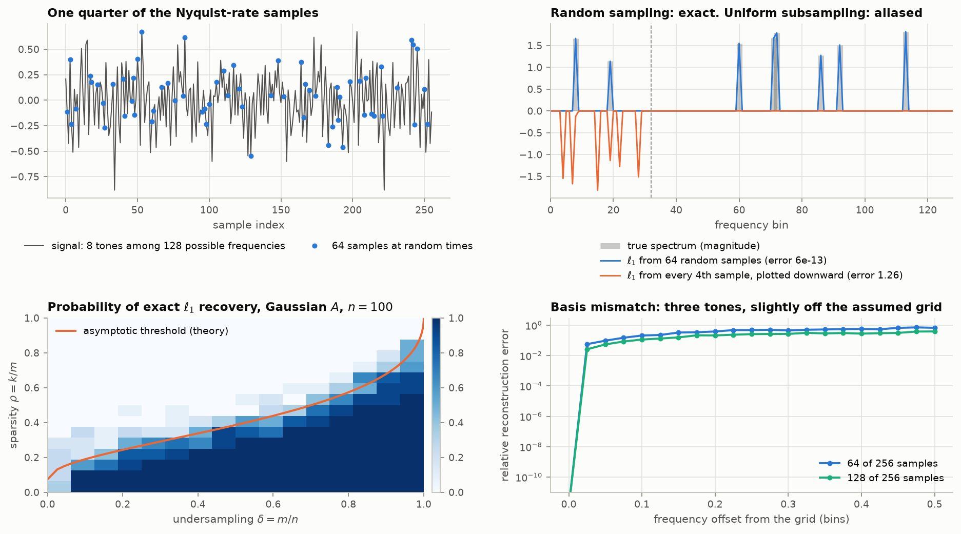
Figure 23. Top: eight tones among 128 possible frequencies, sampled at 64 random instants out of 256 (one quarter of the Nyquist-rate samples). $\ell_1$ minimization recovers the spectrum to $10^{-12}$. The same number of samples taken uniformly (every fourth) fails completely: every tone above the dashed line has folded to below it. Random sampling works because it makes aliases incoherent. Bottom left: empirical probability of exact recovery for Gaussian measurements, $n=100$, with the theoretical asymptotic threshold. Bottom right: the same experiment with three tones displaced from the frequency grid; an offset of 0.025 bins raises the error from $10^{-12}$ to 5%. [Code]

Limits and criticisms, each of which is a failure mode in the spirit of this article:

• Basis mismatch. Real frequencies, delays and positions do not lie on a grid. An off-grid tone is not sparse in the DFT basis, and the guarantees fail abruptly (Figure 23, bottom right) [Chi 2011]. This motivated gridless methods (Section 10 ).
• Noise folding. A compressive measurement that reduces the rate by a factor $\rho$ folds input noise from the whole band into the measurements: 3 dB of SNR lost per octave of subsampling [Davenport 2012; Arias-Castro 2011]. Compressive wide-band receivers trade sensitivity for bandwidth; they do not get both.
• Model fragility. The gain exists only for signals that really are sparse. Conventional sampling degrades gracefully when its model (band-limiting) is slightly wrong; sparse recovery can fail abruptly.
• Computation and structure. Recovery is an optimization problem per acquisition. In imaging, the practical gains came from structured variable-density sampling matched to the structure of wavelet coefficients, for which the classical uniform-random theory is the wrong model [Adcock 2017].
• Hardware. The random demodulator [Tropp 2010] and the modulated wideband converter [Mishali 2010] realize sub-Nyquist acquisition for spectrally sparse signals: total rate about $2NB$ for $N$ bands of width $B$ with unknown positions, against $NB$ if the positions were known and $2f_{\max}$ for Nyquist. Compressed-sensing MRI [Lustig 2007] is the largest deployed application.

---

10. Beyond band-limiting III: parametric signals, super-resolution, and other acquisition models

10.1 Finite rate of innovation

Vetterli, Marziliano and Blu asked the degrees-of-freedom question directly [Vetterli 2002]. A stream of $K$ Diracs per period $\tau$ has $2K$ unknowns per period (locations and amplitudes): a rate of innovation $\rho=2K/\tau$. It is as far from band-limited as a signal can be, and yet $2K+1$ samples per period of its low-pass-filtered version determine it exactly. The low-pass samples give $2K+1$ Fourier coefficients $X[m]=\sum_k a_ku_k^m$, $u_k=e^{-2\pi it_k/\tau}$, a sum of $K$ exponentials; the filter with roots $u_k$ annihilates the sequence, and finding it is Prony’s 1795 method. The same idea handles non-uniform splines, piecewise polynomials and pulse streams, and works with compactly supported kernels that reproduce polynomials or exponentials, which connects it to Strang–Fix [Dragotti 2007].

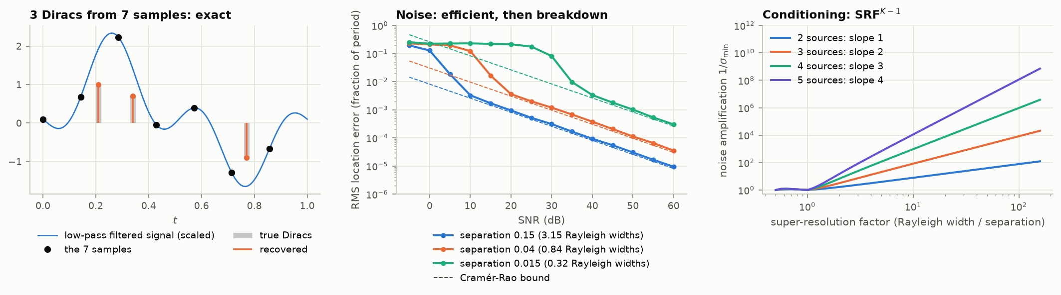
Figure 24. Left: three Diracs recovered exactly (to $10^{-16}$) from seven samples of a low-pass version in which they are not separately visible. Center: with noise, the location error follows the Cramér–Rao bound down to a threshold SNR and then breaks down abruptly; the threshold rises steeply as the spikes approach each other (about 10 dB at 3 Rayleigh widths, 35 dB at 0.3). Right: the cause. The noise amplification $1/\sigma_{\min}$ of the underlying Vandermonde system grows as $\mathrm{SRF}^{K-1}$ for $K$ sources within one resolution cell. [Code]

10.2 Super-resolution theory

When can point sources be resolved below the classical limit $1/f_c$ set by the highest measured frequency?

• Well-separated sources: if the minimum separation is at least $2/f_c$ (improved to $1.26/f_c$), total-variation-norm minimization over measures recovers the sources exactly, with no grid [Candès 2014; Fernandez-Granda 2016]; the atomic-norm formulation does the same from random samples [Tang 2013].
• A sharp threshold: with cut-off $m>1/\Delta+1$ the matrix-pencil method is stable; with $m<(1-\epsilon)/\Delta$ there are pairs of $\Delta$-separated signals that no method can distinguish even at exponentially small noise [Moitra 2015].
• Closely spaced sources: resolution below the Rayleigh limit is possible only at a price in SNR. For $p$ sources clustered within one Rayleigh cell and super-resolution factor $\mathrm{SRF}$, the minimax error scales as $\mathrm{SRF}^{2p-1}\varepsilon$ for amplitudes and $\mathrm{SRF}^{2p-2}\varepsilon/\Omega$ for positions [Donoho 1992; Demanet 2015; Batenkov 2021; Li 2021].

So “beating the diffraction limit” is not forbidden; it costs $\mathrm{SNR}\gtrsim\mathrm{SRF}^{2p-1}$. Two sources at one-tenth the Rayleigh distance need on the order of 60 dB. This is the same exponential ill-conditioning as the prolate tail (Figure 1), gap filling (Figure 16) and superoscillation (Figure 19). Localization microscopy (PALM/STORM) succeeds by changing the model so that $p=1$: emitters are made to blink so that each frame contains isolated sources, and a single source can be localized to $\sigma_{\text{PSF}}/\sqrt{N_{\text{photons}}}$.

10.3 Unlimited (modulo) sampling

A conventional converter clips. A self-reset converter folds the input into $[-\lambda,\lambda)$ instead, and records $y_n=\mathcal M_\lambda(g(nT))$. Bhandari, Krahmer and Raskar showed that a band-limited $g$ with maximum angular frequency $\Omega$ can be recovered from the folded samples alone whenever

$$T\le\frac{1}{2\Omega e},$$

independent of the amplitude of $g$ relative to $\lambda$ [Bhandari 2020]. The mechanism: high-order finite differences of a sufficiently oversampled band-limited signal are small, so $\Delta^Ny$ and $\Delta^Ng$ agree modulo $2\lambda$, and the residual, which takes values in $2\lambda\mathbb Z$, can be integrated back up. In fact any rate above Nyquist suffices for uniqueness [Romanov 2019]; a prototype converter exists [Bhandari 2021]. The sufficient oversampling factor has since been tightened: it falls from $2\pi e$ toward $\pi$ as the order of the differences grows, with a noise-aware condition and a hardware prototype reaching an amplitude expansion of $\rho=108$ [Yan 2025, Theorem 1].

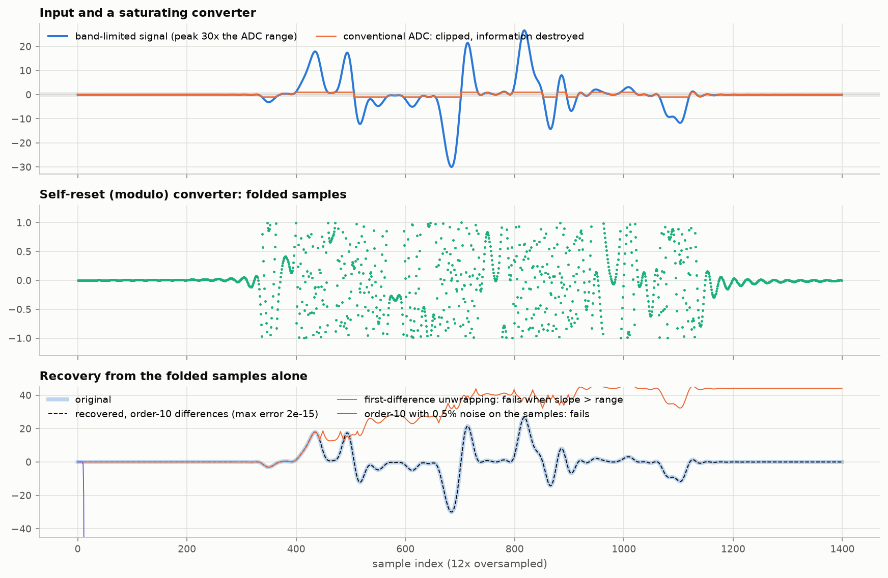
Figure 25. A band-limited signal with peaks 30× the converter range. Top: a clipping converter destroys it. Middle: modulo samples. Bottom: recovery from the folded samples using differences of order 10 (the order prescribed by the theory for this amplitude and 12× oversampling) is exact to rounding error; first-order unwrapping fails as soon as the signal moves by more than the range in one sample; and the high-order method fails with 0.5% noise on the samples, because an $N$-th difference amplifies noise by up to $2^N$. This implementation assumes the record starts unfolded. [Code]

The noise sensitivity in the last panel is not incidental. A March 2026 result shows that recovery from folded samples on an equispaced grid is inherently unstable in the absence of side information, and that an a-priori energy bound restores stability [Romero 2026]. Dynamic range has been traded for conditioning, and the generic lesson of this article applies: uniqueness theorems are cheap, stability is what must be paid for. Recent work reduces the price with a 1-bit folding indicator [Bernardo 2025] and extends the idea to multiband signals at sub-Nyquist rates [Shtendel 2025]. The same effort includes a generalized nonlinear operator that contains clipping, modulo and companding as special cases, for which a band-limited signal is identifiable if and only if the rate exceeds the Nyquist rate [Azar 2022, Theorem 1]; a multi-dimensional theory with a probabilistic guarantee under Gaussian noise [Florescu 2022, Theorem 3]; and modulo sampling on general lattices, where a hexagonal lattice lowers the mean squared error by about 17% in two dimensions [Kvich 2026, Theorem 1].

10.4 Other acquisition models

• Time encoding (integrate-and-fire). Record when an integrator crosses a threshold rather than what the signal is at clock ticks. A band-limited signal is recoverable if consecutive spikes are closer than the Nyquist period [Lazar 2004; overview in Lazar 2005]: a non-uniform sampling theorem in which the signal chooses the sample times. The result extends to shift-invariant spaces under a density condition and survives quantization of the spike times [Gontier 2012 †]; a hardware integrate-and-fire sampler working below the Nyquist rate on finite-rate-of-innovation signals has been built [Naaman 2023 †], and an encoder whose bias adapts to the signal amplitude improves the rate–distortion trade [Omar 2024 †]. Event cameras are a spatial array of such encoders, and a sampling theory for them in shift-invariant spaces now exists [Kamath 2023].
• One-bit and sign measurements. Sigma-delta (Section 4.4 ) is the band-limited case. For sparse vectors, $M$ sign measurements give error no better than $\Omega(K/M)$ [Jacques 2013]: amplitude information is gone and accuracy improves only polynomially.
• Phaseless sampling. A real band-limited function is determined up to sign by $|f(t_n)|$ at more than twice the Nyquist rate [Thakur 2011], but phase retrieval in infinite dimensions is never uniformly stable [Alaifari 2019], and for the short-time Fourier transform no window and no lattice give uniqueness at all [Grohs 2022].
• Dynamical and mobile sampling. Trade spatial samples for temporal ones by sampling an evolving field $A^\ell f$ at few locations [Aldroubi 2017], or sample along the trajectories of moving sensors.
• Information-theoretic limits. For an i.i.d. source with a discrete–continuous mixed distribution, the minimal linear measurement rate for almost-lossless recovery is its Rényi information dimension , the weight of the continuous part, with no logarithmic factor [Wu–Verdú 2010]: the fundamental limit that compressed sensing approaches.

10.5 The pattern

Model	Degrees of freedom	Measurements needed	Reconstruction	What it costs
Band-limited, $2W$	$2WT$	$2WT$	linear	nothing: orthonormal
Shift-invariant space	$T/h$	$T/h$	linear, plus digital filter	approximation error $h^L$
Multiband, known support	$	S	,T$	$
Multiband, unknown support	same	$2	S	,T$
$k$-sparse in a basis	$k$	$\sim k\log(n/k)$	convex optimization	log factor; mismatch; noise folding
Finite rate of innovation	$\rho T$	$\rho T+1$	root finding	SNR threshold
Super-resolved clusters	$2p$ per cell	Fourier data to $f_c$	non-linear	SNR $\sim\mathrm{SRF}^{2p-1}$
Modulo (unlimited)	$2WT$	$2\pi e\times$ (original theory; toward $\pi\times$ [Yan 2025, Theorem 1]), $>1\times$ (uniqueness)	differences and rounding	noise $\times2^N$; unstable without side information

In every row the measurement count tracks the degrees of freedom; what varies is the conditioning and the fragility of the model.

---

11. Recent results (2020–2026)

A selection, emphasizing what changes the picture rather than what refines constants.

Stability results are overtaking uniqueness results.

• Unlimited sampling on a uniform grid is inherently unstable; an energy bound repairs it [Romero 2026].
• Correlated (autoregressive) clock jitter defeats stable sampling at the critical density even though the density condition holds [Gerosa 2026 †].
• Sharp rates for recovery from a finite window of oversampled data: for $f$ band-limited to $[-\delta,\delta]$ with $\delta<\pi$, the worst-case error of optimal recovery from the samples $f(j)$, $|j|\le n$, is of exact order $n^{-1/2}\tan^{2n}(\delta/4)$, which improves on the previous best $O(n^{-1/2}e^{-(\pi-\delta)n})$; from one-sided samples the rate is $\sin^n(\delta/2)$ [Huang 2026, abstract]. This is the precise form of Section 3.3 ’s “oversampling buys a fast-decaying kernel”.
• Computational resolution limits for line spectra: separate thresholds, each with a phase transition, for detecting the number of sources and for stably recovering their positions (Liu and Zhang, 2021); Prony’s method is min-max optimal for clustered nodes and numerically stable [Katz 2023].
• Deep-learning reconstruction: networks trained for accelerated imaging are unstable to tiny perturbations, can miss small structural changes, and can get worse with more samples [Antun 2020]; there are well-conditioned inverse problems for which accurate networks exist but no algorithm can compute them [Colbrook 2022]; over-performance on a few images forces hallucination or instability [Gottschling 2025].

Learned priors replace sparsity, with theorems.

• For a generative prior $G:\mathbb R^k\to\mathbb R^n$ with $d$ ReLU layers, $m=O(kd\log n)$ Gaussian measurements suffice [Bora 2017]; posterior sampling is near-optimal for any prior [Jalal 2021]; but posterior sampling with diffusion models can be computationally intractable in the worst case [Gupta 2024]. A recovery theory that treats diffusion denoisers as time-varying projections onto a low-dimensional model set gives convergence rates under a restricted isometry condition [Leong 2025 †], and posterior sampling has recovery guarantees for one-bit measurements, robust to mismatch of the learned prior [Ma 2026 †].
• Diffusion-model denoisers turn out to perform shrinkage in geometry-adaptive harmonic bases [Kadkhodaie 2024]: the learned prior rediscovers the adapted-basis idea of Section 9.2 .

Aliasing inside neural networks. Strided convolutions and pointwise non-linearities are a sampling chain with no anti-alias filter and with a bandwidth-expanding non-linearity (Section 5.4 , exactly). Consequences and repairs: loss of shift-invariance in classifiers and its restoration by blurring before subsampling [Zhang 2019; Azulay 2019]; texture “sticking” in GANs, removed by treating feature maps as continuous band-limited signals and applying non-linearities at a higher sampling rate [Karras 2021]; the same program for vision transformers [Michaeli 2025] and latent diffusion models [Zhou 2025]. Further repairs: alias-free U-Nets that are equivariant to sub-pixel translation [Scanvic 2026 †], pooling done in the Fourier domain to avoid both aliasing and sinc ringing [Grabinski 2023 †], and low-pass-then-subsample generalized to finite groups for equivariant networks [Rahman 2025 †]. Aliasing has also been proposed as a driver of adversarial vulnerability [Rodríguez-Muñoz 2022 †].

Sampling theory for neural representations. Coordinate networks have a spectral bias toward low frequencies, controllable by Fourier features [Tancik 2020] or periodic activations [Sitzmann 2020], and can be built with an analytically band-limited spectrum [Lindell 2022]; a first exact-recovery theory for fitting such networks to low-pass samples has appeared [Najaf 2024]. Neural rendering re-learned prefiltering: cone tracing in Mip-NeRF [Barron 2021], and in Gaussian splatting a 3-D smoothing filter bounded by the sampling rate of the training views [Yu 2024]. Neural fields with filtering built in: a heat-equation formulation that makes the output anti-aliased at any scale [Becker 2023 †], and band-limited fields for levels of detail [Shabanov 2024 †].

Bits rather than samples. Analog-to-digital compression theory (Section 4.5 ) [Kipnis 2018]; modulo sampling with quantization guarantees [Bernardo 2025]. Sigma-delta and distributed noise shaping applied to samples taken at random points, with error bounds that hold with high probability uniformly over band-limited signals [Joy 2023, Theorem 6.3]. Rate–distortion functions for sampled cyclostationary Gaussian processes [Tan 2024 †]. For one-bit compressed sensing of approximately sparse signals, a lower bound of order $(k/m)^{1/3}$ now matches the best known upper bound [Chen 2026 †]. The first stability guarantees for one-bit sigma-delta beyond first order that beat the classical $\ell^1$ condition have appeared [Joy 2026 †].

Events and time encoding. Event sensors viewed as time-encoding machines for band-limited video: the spike times determine the video exactly, with probability one, once the spikes summed over pixels exceed the number of unknowns, so spatial density buys temporal resolution [Adam 2022, Theorem 1]. Non-uniform sampling whose local gap adapts to the local energy of the signal converges geometrically even with gaps above the Nyquist period in slowly varying regions [Yashaswini 2026, Theorem 1].

Numerical sampling theory. Regularized Shannon formulas with sinh-type and Kaiser–Bessel windows decay at twice the exponential rate of the Gaussian window [Kircheis 2025 †], the constructive counterpart of Section 3.3.

Not found. No general survey of sampling theory since about 2015; the nearest are a review of noise-shaping quantization (Chou and co-authors 2015) and Kircheis, Potts and Tasche’s study of numerical realizations of the theorem (2023). No result sends linear, stable sampling below the Landau rate. The recent literature on time encoding, quantization, modulo sampling and generative priors is growing quickly and was sampled, not exhausted.

---

12. Gotchas and teaching examples

Each of these is a compact demonstration for engineers who know the slogan “sample at twice the highest frequency”. The figures are the ones above.

1. “Twice the highest frequency” is not enough. Sample a sine at exactly $f_s/2$: you get $\sin\varphi\,(-1)^n$, and at $\varphi=0$, silence (Figure 5). The theorem needs strictly more than two samples per cycle, and in practice a guard band sized by the reconstruction filter you can afford (Figure 6).

2. The samples look wrong and are right. A tone at $0.47f_s$ plotted with straight lines appears amplitude-modulated (Figure 5). Nothing is wrong with the data; the plotting program’s linear interpolation is the wrong reconstruction filter. Corollary: never judge a sampled signal’s peak level or shape by eye from raw samples.

3. Digital audio is not a staircase (Figure 12). The stair-step is the zero-order hold inside the DAC, before its filter. Corollary: more bits do not give “smaller steps”; they give a lower noise floor.

4. Samples that never clip can clip (Figure 7): +3 dB for an $f_s/4$ tone, and unbounded in the worst case. Leave headroom or measure true peak.

5. Dither: adding noise removes distortion (Figure 8). A 1.5 LSB sine without dither is a harmonic mess; with dither it is a clean sine in noise, and a sine smaller than one LSB, which vanishes without dither, is recoverable by averaging. This is the best single demonstration that quantization error is not noise unless you make it so.

6. Clock quality beats bit depth at high frequency (Figure 11): a “16-bit” converter with 1 ps of jitter is a 10-bit converter at 100 MHz.

7. Band-limited in, not band-limited out (Figure 14). Any non-linearity (clip, rectify, multiply, compress) makes new frequencies that alias. Oversample around non-linear operations.

8. Aliasing folds noise too. Undersampling a narrow band is legitimate (Figure 15), but all the noise in every folded zone arrives in band. An ADC with 1 GHz input bandwidth clocked at 100 MS/s collects ten zones of noise.

9. Leakage is not aliasing. A tone that does not complete a whole number of cycles in the FFT window spreads across bins. That is truncation in time (convolution with the window’s transform), not folding, and is cured by a window, not by a higher sampling rate.

10. Two-dimensional aliasing is geometric (Figure 4): spurious ring systems appear at definite places. Downsizing an image by dropping pixels, or by bilinear interpolation without a prefilter, produces moiré on fine regular texture such as fabric, brick and screens.

11. A gray scene can come out colored (Figure 26). A Bayer sensor samples red and blue at half the linear density of the full grid; luminance detail between the color and luminance Nyquist limits demosaics to false color. The optical low-pass filter trades it for sharpness.

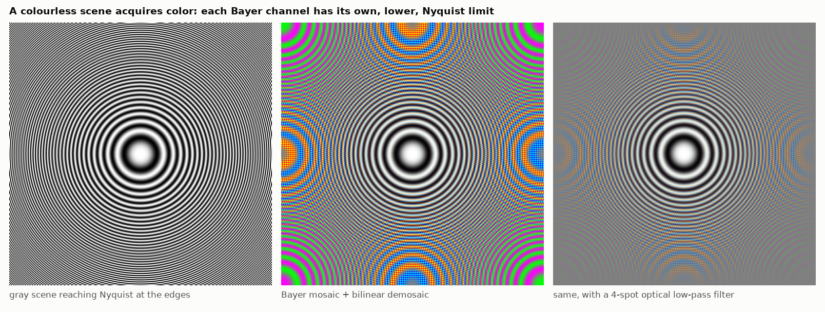
Figure 26. A colorless zone plate, a simulated Bayer mosaic with bilinear demosaicing, and the same with a four-spot optical low-pass filter. [Code]

12. Time aliasing: wagon wheels and propellers. A wheel with $k$ spokes turning at $r$ rev/s filmed at $f$ frames/s appears to turn at the alias of $kr$ modulo $f$. With a rolling shutter each row is its own sampling instant and the image is a space–time slice (Figure 27).

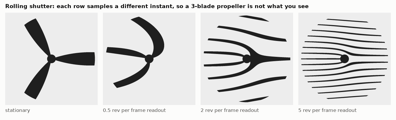
Figure 27. A three-blade propeller under a rolling shutter at four rotation speeds. [Code]

13. Irregular sampling has no simple Nyquist frequency (Figure 17), and random sampling converts aliases into noise (Figure 18). Astronomers, renderers and compressed-sensing designers use this deliberately; satellite altimetry suffers the opposite, with a 9.9156-day repeat orbit aliasing the 12.42-hour $M_2$ tide to about 62 days.

14. The same average rate can be useless (Figure 16). Bunched samples and gaps satisfy the density requirement and are numerically worthless. “We have enough samples” is a statement about counting, not conditioning.

15. Band-limited functions can wiggle arbitrarily fast (Figure 19), at an exponential cost in amplitude. Any scheme promising resolution beyond the band limit from noisy data is paying that cost somewhere.

16. Sub-Nyquist is not sub-information. Compressed sensing recovers eight tones from a quarter of the Nyquist samples (Figure 23) because the signal has 16 degrees of freedom, not 256. Move the tones off the grid by 2.5% of a bin and it fails. The model was carrying the load.

17. Exact in theory, unstable in practice is the commonest pattern in the subject: gap filling, zero-crossing reconstruction, super-resolution of clusters, high-order modulo unwrapping, phase retrieval. Ask of any sampling claim: what is the condition number?

18. Your image viewer resamples. A figure that demonstrates aliasing can acquire new aliasing when displayed at other than 100% (Figure 4’s caption). Test patterns must be viewed pixel-for-pixel.

12.1 Gotchas found in the textbooks and papers

Reading the standard textbooks and papers side by side turns up several that are worth teaching because the sources themselves disagree:

19. The books disagree about the history. Unser places Shannon’s “common knowledge in the communication art” remark in the 1949 paper and Vetterli–Kovačević–Goyal in the 1948 one; Mallat says the theorem was “first proved by Whittaker … in 1935” (that is J. M. Whittaker’s book; E. T. Whittaker’s paper is 1915); Smith’s DSP guide credits “authors of 1940s papers”; Salomon says it “was proved by Harry Nyquist”. Meijering notes that the often-repeated Cauchy 1841 attribution is false.

20. “Nyquist rate” and “Nyquist frequency” are not used consistently. Vetterli: the Nyquist rate is a property of the signal (twice its bandwidth) and the Nyquist frequency a property of the system (half the sampling rate). PBRT calls the minimum sampling frequency the Nyquist frequency; Smith’s verdict is “It depends who you ask!”. Define both on first use in anything you write.

21. $\ge$ against $>$. Numerical Recipes states the theorem with the spectrum vanishing for $|f|\ge f_c$ and then advises “at least two points per cycle”; Horowitz and Hill say “equal to twice”; Grafakos gives the careful $L^1$ statement and the all-zero-samples counterexample as an exercise.

22. Sinc is not the practical ideal. Windowed sincs have approximation order zero (they do not reproduce a constant, so image brightness drifts with position) [Thévenaz 2000]; Unser’s own first complaint about the theorem is that the reconstruction formula “is rarely used in practice (especially with images) because of the slow decay of the sinc function” [Unser 2000].

23. “Cubic B-splines blur” is an implementation error: using the samples as spline coefficients instead of running the prefilter. Hou and Andrews already labeled the blurry result “with incorrect coefficients” in 1978.

24. Interpolating kernels are not optimal. Insisting that the kernel itself pass through the samples costs an order of approximation (Keys: order 3; cubic B-spline with prefilter: order 4, same support). In Nehab and Hoppe’s benchmark the Mitchell–Netravali filter, chosen by subjective testing, ranks near the bottom on SSIM (0.715, against 0.857 for Catmull-Rom and 0.935 for the interpolating cubic B-spline) [Nehab 2014, Table 10.1].

25. $6.02N+1.76$ dB is a full-scale-sine figure. For Gaussian-like audio with sensible headroom Zölzer derives $6.02w-8.5$ dB.

26. Aliasing as a feature. A phone gyroscope sampled at 200 Hz recovers speech content through aliasing (Gyrophone, USENIX Security 2014); multi-frame super-resolution requires aliased frames (Wronski et al. 2019); image-scaling attacks hide a second image in the pixels that a non-antialiasing resizer happens to pick (Quiring et al. 2020).

27. A slice of a band-limited function is not band-limited. A 2-D slice through 3-D band-limited noise contains all lower frequencies (Cook and DeRose, Wavelet Noise, 2005).

28. Sampling is not quantization. Gleick’s The Information has a signal “discretized without loss as per the Shannon sampling theorem”; the theorem discretizes time only.

---

13. Conclusions

What the theorem is. An orthonormal expansion in one particular reproducing-kernel Hilbert space, used by Shannon to count dimensions. It is exact, and it is exactly conditioned, for finite-energy signals with exact samples.

Where it stops. In order of how often it matters in practice:

1. Signals are not band-limited, so the question is always how much error, and that is governed by spectral decay (Section 2 ) or, in a better-chosen space, by approximation order (Section 8 ).
2. Samples are finite-precision. The $\Delta^2/12$ noise model is a theorem with hypotheses (Widrow), dither is how one enforces them, and the proper accounting is in bits: rate and resolution trade against each other with exchange rates that range from half a bit per octave (PCM) to exponential (optimal 1-bit schemes), under an entropy bound (Section 4 ).
3. Timing is finite-precision, which caps SNR by input frequency (Section 5 ).
4. Kernels must have finite support, which is impossible at the critical rate without paying in truncation error, ringing or instability; a guard band buys an absolutely summable kernel and with it stability in the sup norm (Section 3 ).
5. Sampling sets must be dense enough (Landau), and density is not conditioning (Section 7 ).

What goes beyond it. Not a faster or cleverer way to sample band-limited signals: for that class, with linear stable reconstruction, $2W$ (more generally the Landau rate) is final. What goes beyond is a different model:

• Other linear subspaces (splines, wavelets, any shift-invariant space), with a digital correction filter and a non-ideal acquisition device: generalized sampling.
• Unions of subspaces: sparsity in a basis or frame (wavelets, curvelets, shearlets), compressed sensing, multiband signals with unknown support.
• Finite-dimensional parametric families: finite rate of innovation, line spectra, point sources.
• Non-linear acquisition: modulo folding, time encoding, one-bit measurements.

Each has its own “sampling theorem” matching measurements to degrees of freedom, and each has a failure mode that plays the role aliasing plays for band-limited signals: basis mismatch, noise folding, SNR thresholds, the $\mathrm{SRF}^{2p-1}$ law, instability without side information.

One idea to keep. Every “beyond Nyquist” claim can be audited with three questions. How many degrees of freedom does the assumed model have? (The measurement count cannot beat that.) What is the condition number of recovery? (Exponentially small eigenvalues are behind every too-good result.) What happens when the model is slightly wrong? (Linear, band-limited sampling fails gently; most of its competitors do not.)

Open ends noted during the research: sharp constants for many classical bounds (truncation, the factor 2 in the aliasing bound) could not be re-verified from primary sources; no general survey of sampling theory has appeared since about 2015 (Eldar’s book), despite the volume of new work in Section 11 ; and a satisfactory theory of sampling for perceptual fidelity, rather than $L^2$ error, does not yet exist (the companion article on image processing takes this up).

---

References

A dagger † marks items whose specific statements, as used here, were confirmed only from an abstract, a secondary source, or memory. [—] marks sources that were not obtained and are cited from secondary sources. A [PDF] link is a copy hosted here; [DOI], [arXiv] and [link] go to the public source.

History and foundations

• [Nyquist 1928] DOI H. Nyquist, “Certain topics in telegraph transmission theory”, Trans. AIEE 47.
• [Kotelnikov 1933] link V. A. Kotelnikov, “On the transmission capacity of ’ether’ and wire in electrocommunications” (English translation).
• [Shannon 1949] DOI C. E. Shannon, “Communication in the presence of noise”, Proc. IRE 37 (1998 Proc. IEEE reprint).
• [Lüke 1999] DOI H. D. Lüke, “The origins of the sampling theorem”, IEEE Commun. Mag. 37(4).
• [Meijering 2002] DOI E. Meijering, “A chronology of interpolation”, Proc. IEEE 90(3), 319–342.
• [Unser 2000] DOI M. Unser, “Sampling—50 years after Shannon”, Proc. IEEE 88(4), 569–587.
• Jerri 1977, “The Shannon sampling theorem—its various extensions and applications: a tutorial review”, Proc. IEEE 65(11). [—]
• Higgins 1985, “Five short stories about the cardinal series”, Bull. AMS 12. [—]
• L. Grafakos, Classical Fourier Analysis, 3rd ed., 2014.
• M. Vetterli, J. Kovačević, V. Goyal, Foundations of Signal Processing, 2014 (chs. 5–7).

Time–frequency limits, convergence, error bounds

• [Slepian 1961 DOI ; Landau 1961 DOI ; Landau 1962 DOI ] Slepian, Pollak, Landau, “Prolate spheroidal wave functions, Fourier analysis and uncertainty” I–III, Bell Syst. Tech. J.
• [Slepian 1976] DOI D. Slepian, “On bandwidth”, Proc. IEEE 64(3), 292–300.
• [Boche 2015] DOI H. Boche, U. Mönich et al., “Strong divergence for system approximations”, arXiv:1505.03057; also [Boche 2013] link , [Boche 2014] DOI .
• [Boche–Mönich 2008] “There exists no globally uniformly convergent reconstruction for the Paley–Wiener space $PW^1_\pi$ of bandlimited functions sampled at Nyquist rate”, IEEE Trans. SP. [—] † (secondary source: H. Boche, V. Pohl DOI , “System approximations and generalized measurements in modern sampling theory”, arXiv:1410.5872. )
• [Butzer 2012] link P. Butzer; R. Stens link , Inzell lecture slides on sampling theory and the aliasing error.
• [Weiss 1963; Brown 1967; Butzer–Splettstösser 1977] aliasing error bound. [—] † (statement checked against [Butzer 2012])
• [Helms–Thomas 1962; Jagerman 1966; Yao–Thomas 1966] truncation error bounds. [—] †
• [Butzer–Splettstösser–Stens 1988] “The sampling theorem and linear prediction in signal analysis”, Jahresber. DMV 90, 1–70. [—] †
• [ITU-R 2023] link Rec. ITU-R BS.1770-5 (true-peak measurement).

Quantization, dither, conversion

• [Bennett 1948] DOI W. R. Bennett, “Spectra of quantized signals”, Bell Syst. Tech. J. 27.
• [Widrow 1996] DOI B. Widrow, I. Kollár, M.-C. Liu, “Statistical theory of quantization”, IEEE Trans. IM 45(2).
• Sripad and Snyder 1977. [—] †
• Gray 1990 “Quantization noise spectra”. [—] †
• Gray and Neuhoff 1998 “Quantization”. [—] †
• [Lipshitz 1992] S. Lipshitz, R. Wannamaker, J. Vanderkooy, “Quantization and dither: a theoretical survey”, J. AES 40(5).
• [Wannamaker 2000] Wannamaker, Lipshitz, Vanderkooy, Wright, “A theory of nonsubtractive dither”, IEEE Trans. SP 48(2). [—] †
• C. Christou, Optimal Dither and Noise Shaping in Image Processing, MMath thesis, Waterloo, 2008.
• U. Zölzer, Digital Audio Signal Processing, 2nd ed., 2008 (chs. 2–3).
• [Thao 1994] DOI N. Thao, M. Vetterli, “Deterministic analysis of oversampled A/D conversion and decoding improvement based on consistent estimates”, IEEE Trans. SP 42(3). (abstract and results pages read as images)
• [Daubechies 2003] DOI I. Daubechies, R. DeVore, “Approximating a bandlimited function using very coarsely quantized data”, Ann. Math. 158. †
• [Güntürk 2003] “One-bit sigma-delta quantization with exponential accuracy”, CPAM 56. [—] (not obtained. The exponent 0.076 is confirmed in [Deift 2011, p. 3] and in Krahmer’s 2009 NYU thesis, pp. 13 and 42. Güntürk’s 2000 Princeton thesis predates the result: its p. 61 gives the best proved rate as $\lambda^{-\beta\log\lambda}$, “far short of any exponential accuracy”)
• [Deift 2011] DOI P. Deift, S. Güntürk, F. Krahmer, “An optimal family of exponentially accurate one-bit sigma-delta quantization schemes”, CPAM 64.
• [Daubechies 2006] DOI Daubechies, DeVore, Güntürk, Vaishampayan, “A/D conversion with imperfect quantizers”, IEEE Trans. IT 52(3).
• [Kipnis 2018] DOI A. Kipnis, Y. Eldar, A. Goldsmith, “Analog-to-digital compression”, IEEE SP Mag. 35(3); “Fundamental distortion limits of analog-to-digital compression DOI ”, IEEE Trans. IT.
• [Chen 2013] DOI Y. Chen, Y. Eldar, A. Goldsmith, “Shannon meets Nyquist: capacity of sampled Gaussian channels”, IEEE Trans. IT 59(8).
• [Neu 2010] link T. Neu, “Clock jitter analyzed in the time domain, Part 1”, TI SLYT379.
• [Walden 1999] R. Walden, “Analog-to-digital converter survey and analysis”, IEEE JSAC 17(4). [—] †
• [Murmann 2022] link B. Murmann, ISSCC 2022 short course slides; ADC Performance Survey.
• R. Lyons, Understanding Digital Signal Processing.
• S. W. Smith, The Scientist and Engineer’s Guide to DSP (ch. 3).
• [Lavry 2004] link D. Lavry, “Sampling theory for digital audio”.
• Analog Devices tutorials MT-001, MT-003, MT-007, MT-008 (W. Kester). [—]

Reconstruction, band-pass and non-uniform sampling

• [Mitchell 1988] DOI D. Mitchell, A. Netravali, “Reconstruction filters in computer graphics”, SIGGRAPH ‘88.
• [Vaughan 1991] R. Vaughan, N. Scott, D. White, “The theory of bandpass sampling”, IEEE Trans. SP 39(9). [—] †
• [Landau 1967] H. Landau, “Necessary density conditions for sampling and interpolation of certain entire functions”, Acta Math. 117. [—] †
• [Papoulis 1977] A. Papoulis, “Generalized sampling expansion”, IEEE Trans. CAS 24. [—] †
• [Cheung–Marks 1985] ill-posedness. [—] †
• [Unser 1997] DOI M. Unser, J. Zerubia, “Generalized sampling: stability and performance analysis”, IEEE Trans. SP 45(12).
• [Mishali 2009] DOI M. Mishali, Y. Eldar, “Blind multiband signal reconstruction”, IEEE Trans. SP 57(3).
• [Logan 1977] DOI B. Logan, “Information in the zero crossings of bandpass signals”, Bell Syst. Tech. J. 56. (theorem statement checked on the page image, printed p. 489)
• [Eyer 1999] DOI L. Eyer, P. Bartholdi, “Variable stars: which Nyquist frequency?”, A&AS 135.
• [VanderPlas 2018] DOI J. VanderPlas, “Understanding the Lomb–Scargle periodogram”, ApJS 236.
• [Ferreira–Kempf 2006] “Superoscillations: faster than the Nyquist rate”, IEEE Trans. SP 54(10). [—] †
• [Kempf 2018] DOI “Four aspects of superoscillations”.
• Kempf 1999 DOI .
• [McEwen 2011] DOI J. McEwen, Y. Wiaux, “A novel sampling theorem on the sphere”, IEEE Trans. SP 59(12).
• Numerical Recipes in C (§12.1, §13.4, §13.8, §13.11).
• f. j. harris DOI , “On the use of windows…”, Proc. IEEE 66(1), 1978.

Generalized sampling and approximation

• [Unser 1994] DOI M. Unser, A. Aldroubi, “A general sampling theory for nonideal acquisition devices”, IEEE Trans. SP 42(11).
• [Blu 1999] DOI T. Blu, M. Unser, “Quantitative Fourier analysis of approximation techniques: Part I”, IEEE Trans. SP 47(10).
• [Nehab 2014] DOI D. Nehab, H. Hoppe, “A fresh look at generalized sampling”, Found. Trends CGV 8(1).
• [Thévenaz 2000] DOI P. Thévenaz, T. Blu, M. Unser, “Image interpolation and resampling”.
• Blu, Thévenaz, Unser, “MOMS” DOI (2001), “Linear interpolation revitalized” DOI (2004).
• Condat, Blu, Unser 2005 DOI .
• Sacht and Nehab 2014 DOI .
• Kybic, Blu, Unser 2002 DOI .
• [Eldar 2009] DOI Y. Eldar, T. Michaeli, “Beyond bandlimited sampling”, IEEE SP Mag. 26(3).
• [Lu 2008] DOI Y. Lu, M. Do, “A theory for sampling signals from a union of subspaces”, IEEE Trans. SP 56(6).
• Y. Eldar, Sampling Theory: Beyond Bandlimited Systems, CUP 2015. [—]
• Graph and topological sampling: [Chen 2015] DOI , [Anis 2016] DOI , [Tanaka 2020] PDF (two papers), [Barbarossa 2020] DOI DOI .

Wavelets, sparsity, compressed sensing

• S. Mallat, A Wavelet Tour of Signal Processing, 2nd ed. (ch. 9).
• [DeVore 1998] R. DeVore, “Nonlinear approximation”, Acta Numerica 7.
• [Donoho 1998] DOI D. Donoho, M. Vetterli, R. DeVore, I. Daubechies, “Data compression and harmonic analysis”, IEEE Trans. IT 44(6).
• [Candès 2004] DOI E. Candès, D. Donoho, “New tight frames of curvelets…”, CPAM 57(2).
• [Kutyniok 2011] DOI G. Kutyniok, W.-Q. Lim, “Compactly supported shearlets are optimally sparse”, J. Approx. Theory 163.
• [Do 2005] DOI contourlets.
• Mallat 2012 DOI , “Group invariant scattering”.
• [Candès 2006a] DOI Candès, Romberg, Tao, “Robust uncertainty principles”, IEEE Trans. IT 52(2); “Stable signal recovery” DOI , CPAM 59(8).
• [Donoho 2006] DOI “Compressed sensing”.
• [Candès 2008] DOI “The restricted isometry property…”.
• [Donoho 2009] DOI Donoho and Tanner, phase transitions.
• [Chi 2011] Chi, Scharf, Pezeshki, Calderbank, “Sensitivity to basis mismatch in compressed sensing”, IEEE Trans. SP 59(5). [—] †
• [Arias-Castro 2011] DOI noise folding.
• [Davenport 2012] DOI “The pros and cons of compressive sensing for wideband signal acquisition”.
• [Tropp 2010] DOI random demodulator.
• [Mishali 2010] DOI modulated wideband converter.
• Mishali and Eldar 2011 arXiv , Duarte and Eldar 2011 DOI (reviews).
• [Lustig 2007] DOI sparse MRI.
• [Jacques 2013] DOI one-bit CS.
• [Adcock 2017] PDF “Breaking the coherence barrier”.
• [Wu–Verdú 2010] “Rényi information dimension”, IEEE Trans. IT 56(8). [—] †

Finite rate of innovation and super-resolution

• [Vetterli 2002] DOI Vetterli, Marziliano, Blu, “Sampling signals with finite rate of innovation”, IEEE Trans. SP 50(6).
• [Dragotti 2007] DOI .
• Blu et al. 2008 DOI , “Sparse sampling of signal innovations”.
• Tur, Eldar, Friedman 2011 DOI .
• [Donoho 1992] “Superresolution via sparsity constraints”, SIAM J. Math. Anal. 23(5). [—] †
• [Candès 2014] DOI Candès and Fernandez-Granda, “Towards a mathematical theory of super-resolution”, CPAM 67(6).
• Candès 2013 DOI (noisy data).
• [Fernandez-Granda 2016] DOI .
• [Tang 2013] DOI .
• [Moitra 2015] DOI .
• [Demanet 2015] arXiv .
• [Batenkov 2021] DOI .
• [Li 2021] DOI .
• [Katz 2023] DOI .

Other acquisition models

• [Bhandari 2020] DOI Bhandari, Krahmer, Raskar, “On unlimited sampling and reconstruction”, IEEE Trans. SP.
• [Romanov 2019] DOI .
• [Bhandari 2021] DOI (prototype ADC).
• Florescu 2022 PDF .
• [Bernardo 2025] PDF .
• [Shtendel 2025] PDF .
• [Romero 2026] arXiv “Stability in unlimited sampling”, arXiv:2603.24425.
• [Lazar 2004] A. Lazar, L. Tóth, “Perfect recovery and sensitivity analysis of time encoded bandlimited signals”, IEEE Trans. CAS-I 51(10). [—] †
• [Kamath 2023] arXiv neuromorphic sampling.
• [Thakur 2011] DOI .
• [Alaifari 2019] PDF .
• [Grohs 2022] PDF (phase retrieval).
• [Aldroubi 2017] arXiv (dynamical sampling).

Learning-era results

• [Antun 2020] DOI .
• [Colbrook 2022] PDF .
• [Gottschling 2025] DOI .
• [Bora 2017] arXiv .
• [Jalal 2021] PDF PDF (two papers).
• [Gupta 2024] PDF .
• [Kadkhodaie 2024] PDF .
• [Zhang 2019] arXiv .
• [Azulay 2019] arXiv .
• [Karras 2021] arXiv .
• [Michaeli 2025] DOI .
• [Zhou 2025] DOI .
• [Tancik 2020] arXiv .
• [Sitzmann 2020] arXiv .
• [Lindell 2022] DOI .
• [Najaf 2024] DOI .
• [Barron 2021] DOI .
• [Yu 2024] DOI .

Additional sources

Read at the level of the abstract only † unless a page is cited in the text.

• [Bailey 2010] PDF B. Bailey, “Sampling and recovery of multidimensional bandlimited functions via frames”, arXiv:1009.2043 (Kadec sequences, p. 17).
• [Kadec 1964] M. Kadec, “The exact value of the Paley–Wiener constant”, Sov. Math. Dokl. 5, 559–561. [—]
• [Al-Hammali 2020] DOI H. Al-Hammali, A. Faridani, “The zeros of a sine-type function and the peak value problem”, Signal Process. 167.
• Wunder and Boche 2003. [—]
• [Gerosa 2026] PDF Gerosa, Eriksson, “Sampling with autoregressive clock jitter”, arXiv:2606.03942.
• [Huang 2026] arXiv Huang, Zhang, “Sharp rates for optimal recovery of bandlimited functions from localized oversampling”, arXiv:2611.11461 (check for later versions).
• [Yan 2025] PDF arXiv:2509.12971.
• [Azar 2022] DOI Azar, Mulleti, Eldar, arXiv:2206.14656.
• [Florescu 2022] PDF Florescu, Bhandari, arXiv:2209.06426.
• [Lazar 2005] Lazar, Simonyi, Tóth, “Time encoding of bandlimited signals, an overview”.
• [Gontier 2012] DOI Gontier, Vetterli, arXiv:1108.3149.
• [Naaman 2023] DOI arXiv:2301.02012.
• [Omar 2024] DOI arXiv:2403.02992.
• [Joy 2023] DOI Joy, Krahmer, Lupoli, Ramakrishnan, arXiv:2306.15758.
• [Tan 2024] DOI arXiv:2405.11405.
• Kipnis, Goldsmith, Eldar, Weissman DOI , “Distortion rate function of sub-Nyquist sampled Gaussian sources”, arXiv:1405.5329.
• [Leong 2025] PDF arXiv:2509.20511.
• [Ma 2026] PDF arXiv:2610.11834.
• Guo et al. 2025, arXiv:2509.03898.
• [Scanvic 2026] PDF arXiv:2603.11323.
• [Rahman 2025] PDF ICLR 2025, arXiv:2504.17258.
• [Grabinski 2023] DOI arXiv:2307.09804.
• [Rodríguez-Muñoz 2022] arXiv arXiv:2212.11760.
• [Becker 2023] PDF Thera, arXiv:2311.17643.
• [Shabanov 2024] DOI BANF, CVPR 2024.
• Vendor notes: Brannon link , Analog Devices AN-756; Vallenilla and Reeder link , Texas Instruments SBAA653.

Further sources used for examples

• Parmar, Zhang, Zhu 2022 DOI , “On aliased resizing…”.
• Quiring et al. 2020, image-scaling attacks.
• Wronski et al. 2019 PDF , handheld multi-frame super-resolution.
• Cook and DeRose 2005 DOI , Wavelet Noise.
• Heckbert 1989 thesis link .
• PBRT ch. 7 link (first edition).
• Michalevsky et al. 2014 link , Gyrophone.
• Lau and Arce, Modern Digital Halftoning.
• Dubois, “Video sampling and interpolation”, in Bovik (ed.).

Sources added in the final pass

• [Kircheis 2023] arXiv M. Kircheis, D. Potts, M. Tasche, “On numerical realizations of Shannon’s sampling theorem” (Sampl. Theory Signal Process. Data Anal. 22, 2024).
• [Kircheis 2025] arXiv “Some remarks on regularized Shannon sampling formulas”. †
• [Trynin 2007] link A. Trynin, “Estimates for the Lebesgue functions and the Nevai formula for sinc-approximations”, Sib. Mat. Zh. 48(5), 1155–1166.
• Wunder and Afrasiabi-Gorgani 2016, “Overshooting and L1-norms of a class of Nyquist filters”, arXiv:1602.08975.
• [Avantaggiati 2016] arXiv A. Avantaggiati, P. Loreti, P. Vellucci, on Kadec’s 1/4 theorem.
• [Adam 2022] arXiv K. Adam, A. Scholefield, M. Vetterli, “How asynchronous events encode video”.
• [Yashaswini 2026] arXiv “Adaptive non-uniform sampling of bandlimited signals via algorithm-encoder co-design”.
• [Kvich 2026] arXiv Y. Kvich, Y. Eldar, “Lattice modulo sampling”.
• [Chen 2026] arXiv “Near-optimal lower bounds on one-bit compressed sensing of approximately sparse signals”. †
• [Joy 2026] arXiv “On trajectory-based stability analysis for 1-bit Sigma-Delta quantization”. †
• Chou, Güntürk, Krahmer, Saab, Yılmaz 2015, “Noise-shaping quantization methods for frame-based and compressive sampling systems”, arXiv:1502.05807.

Code

• [Code] Private test code written for these articles: figure generation, simulations and numerical checks. It is not published.